Explore Rehabilated Non-Functional Water Points in Nigeria

Published

December 25, 2022

1. OVERVIEW

1.1 Objectives

  • Explore the relationship between non-functional water points and other attributes.

1.2 Study Area Introduction

Alpha-3 Code : NGA

Population : 225 million (1st in Africa, 6th globally)

Local Government Areas (LGA) : 774

Water Point Observations : 95,008

Environmental Aspects :

  • Geography :

    • Southwest - “rugged” highland.

    • Southeast - hills and mountains, which form the Mambilla Plateau, the highest plateau in Nigeria.

  • Hydrology :

    • Two (2) main catchment areas - Chad Basin & Niger catchment area.

    • Surface area of lake Chad is shrinking recent decades due to irrigation activities.1

    • Untreated wastes dump in places resulted in waterways and groundwater pollution.2

  • Vegetation Coverage :

    • Lost nearly 80% of primary forest by 2012.3

    • States with dense forests concentrated : Bayelsa, Cross River, Edo, Ekiti, Ondo, Osun, Rivers, and Taraba.

  • 1 Wikipedia. Nigeria. https://en.wikipedia.org/wiki/Nigeria

  • 2 Ogbonna, D.N., Ekweozor, I.K.E., Igwe, F.U. (2002). “Waste Management: A Tool for Environmental Protection in Nigeria”. Ambio: A Journal of the Human Environment. 31 (1): 55–57. doi:10.1639/0044-7447(2002)031[0055:wmatfe]2.0.co;2.

  • 3 https://rainforests.mongabay.com/20nigeria.htm

  • 1.3 Scope of Works

    • Explore the non-functional water points that recently rehabilitated.

    2. R PACKAGE REQUIRED

    2.1 Load R Packages

    Usage of the code chunk below :

    p_load( ) - pacman - to load packages. This function will attempt to install the package from CRAN or pacman repository list if its found not installed.

    Show the code
    pacman::p_load(sf, tidyverse, questionr, janitor, psych, ggplot2, gcookbook, tmap, ggpubr, egg, corrplot, gtsummary, regclass, caret, heatmaply, ggdendro, cluster, factoextra, spdep, ClustGeo, GGally, skimr, stringr, funModeling, knitr, caTools, viridis, rgeoda)

    3. GEOSPATIAL DATA

    3.1 Acquire Data Source

    Note

    The file size of the downloaded data is about 422 MB due to water points data from multiple countries.

    • Such file size may require extra effort and time to manage the code chunks and files in the R environment before pushing them to GitHub.

    Hence, to avoid any error in pushing files larger than 100 MB to Git, filtered Nigeria water points and removed unnecessary variables before uploading into the R environment.

    Therewith, the CSV file size should be lesser than 100 MB.

  • 4 Runfola, D. et al. (2020) geoBoundaries: A global database of political administrative boundaries. PLoS ONE 15(4): e0231866. https://doi.org/10.1371/journal.pone.0231866

  • 3.2 Import Attribute Data

    Four (4) data frames to be created for different context, i.e.

    • wp_coord = coordinated related variables.

    • wp_cond = status and conditions related variables.

    • wp_adm = administrative and measurements related variables.

    • wp = master file that combine all three (3) data frames above.

    3.2.4 Create Master File

    Show the code
    wp3 <- left_join(
      (left_join
       (wp_coord3,wp_cond3,
         by = c("row_id")
         )),
      wp_adm3, 
      by = c("row_id"))

    3.2.5 Convert Well Known Text (WKT) Data to SF Data Frame

    • The “New Georeferenced Column” in wp_rds contains spatial data in a WKT format.

    • Two (2) steps to convert the WKT data format into an sf data frame.

    3.2.5.1 derive new field :: “geometry”

    Show the code
    wp3$geometry = st_as_sfc(wp3$`New Georeferenced Column`)

    3.2.5.2 convert to SF Data Frame

    Show the code
    wp3_sf<- st_sf(wp3, crs = 4326)
    st_crs(wp3_sf)
    Coordinate Reference System:
      User input: EPSG:4326 
      wkt:
    GEOGCRS["WGS 84",
        ENSEMBLE["World Geodetic System 1984 ensemble",
            MEMBER["World Geodetic System 1984 (Transit)"],
            MEMBER["World Geodetic System 1984 (G730)"],
            MEMBER["World Geodetic System 1984 (G873)"],
            MEMBER["World Geodetic System 1984 (G1150)"],
            MEMBER["World Geodetic System 1984 (G1674)"],
            MEMBER["World Geodetic System 1984 (G1762)"],
            MEMBER["World Geodetic System 1984 (G2139)"],
            ELLIPSOID["WGS 84",6378137,298.257223563,
                LENGTHUNIT["metre",1]],
            ENSEMBLEACCURACY[2.0]],
        PRIMEM["Greenwich",0,
            ANGLEUNIT["degree",0.0174532925199433]],
        CS[ellipsoidal,2],
            AXIS["geodetic latitude (Lat)",north,
                ORDER[1],
                ANGLEUNIT["degree",0.0174532925199433]],
            AXIS["geodetic longitude (Lon)",east,
                ORDER[2],
                ANGLEUNIT["degree",0.0174532925199433]],
        USAGE[
            SCOPE["Horizontal component of 3D system."],
            AREA["World."],
            BBOX[-90,-180,90,180]],
        ID["EPSG",4326]]
    3.3 Import Boundary Data

    Show the code
    bdy_nga <- st_read(dsn = "data/geospatial",
                   layer = "geoBoundaries-NGA-ADM2",
                   crs = 4326) %>%
      select(shapeName)
    
    problems(bdy_nga)

    3.3.1 save and read RDS file :: wp_adm

    Show the code
    write_rds(bdy_nga,"data/geodata/bdy_nga.rds",compress = "xz")
    bdy_nga <- read_rds("data/geodata/bdy_nga.rds")

    3.3.2 Review Imported File

    3.3.2.1 check for missing and duplicated data

    Show the code
    skim(bdy_nga)
    Warning: Couldn't find skimmers for class: sfc_MULTIPOLYGON, sfc; No
    user-defined `sfl` provided. Falling back to `character`.
    Data summary
    Name bdy_nga
    Number of rows 774
    Number of columns 2
    _______________________
    Column type frequency:
    character 2
    ________________________
    Group variables None

    Variable type: character

    skim_variable n_missing complete_rate min max empty n_unique whitespace
    shapeName 0 1 3 18 0 768 0
    geometry 0 1 878 33370 0 774 0

    Remarks :

    • There is no missing data.

    • Under “n_unique”, there is 774 unique “geometry” but only 768 unique “shapeName”.

      • That’s mean there are 6 values of “shapeName” duplicated among the identified unique shapeNames.

    3.3.2.2 list the unique “shapeName” associated with duplication

    Show the code
    dupl_shapeName <- bdy_nga %>%
      add_count(bdy_nga$shapeName) %>%
      filter(n!=1) %>%
      select(-n)
    
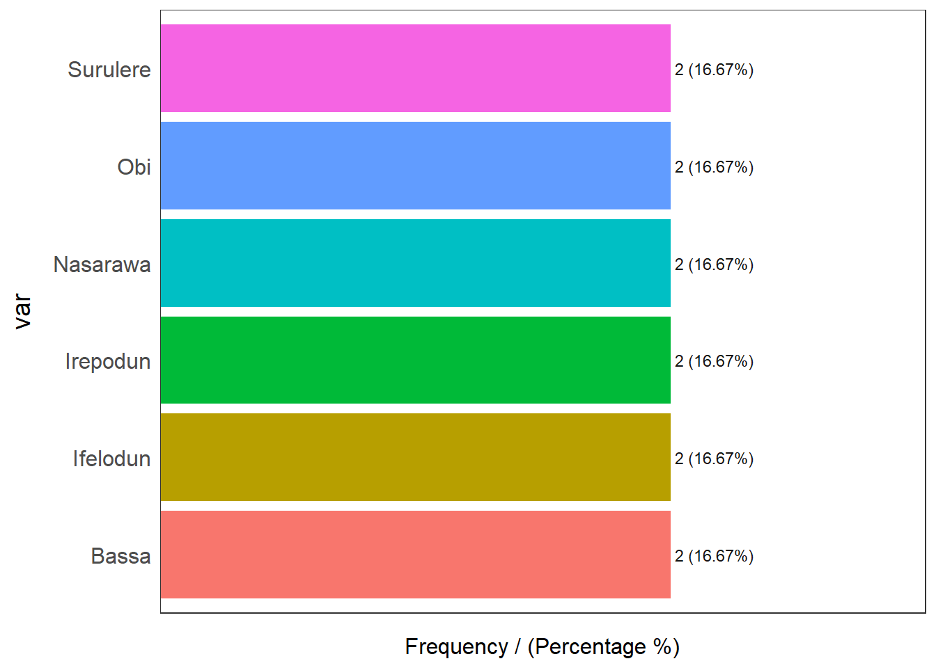
    freq(dupl_shapeName$shapeName)
    Warning: The `<scale>` argument of `guides()` cannot be `FALSE`. Use "none" instead as
    of ggplot2 3.3.4.
    ℹ The deprecated feature was likely used in the funModeling package.
      Please report the issue at <https://github.com/pablo14/funModeling/issues>.

           var frequency percentage cumulative_perc
    1    Bassa         2      16.67           16.67
    2 Ifelodun         2      16.67           33.34
    3 Irepodun         2      16.67           50.01
    4 Nasarawa         2      16.67           66.68
    5      Obi         2      16.67           83.35
    6 Surulere         2      16.67          100.00

    3.3.2.3 verify findings in section 3.3.1.2

    Show the code
    tmap_mode("view")
    tmap mode set to interactive viewing
    Show the code
    tm_shape(bdy_nga)+
      tm_polygons()+
      tm_view(set.zoom.limits = c(6,8))+
    
    tm_shape(dupl_shapeName)+
      tm_fill("shapeName",
              n = 6,
              style = "jenks")+
      tm_borders(alpha = 0.5)+
      tmap_style("albatross")+
      tm_layout(main.title = "Distribution of Duplicated ShapeName",
                main.title.size = 1.3,
                main.title.position = "center")
    tmap style set to "albatross"
    other available styles are: "white", "gray", "natural", "cobalt", "col_blind", "beaver", "bw", "classic", "watercolor" 
    Show the code
    tmap_mode("plot")
    tmap mode set to plotting

    Remarks :

    The plot above indicates those duplicated water points are not within the same location.

    3.3.2.4 acquire State info for duplicated value

    The State info to be combined with the duplicated “shapeName”. This will make all the shapeName unique.

    Show the code
    dupl_shapeName %>%
      mutate(st_centroid(
        dupl_shapeName$geometry, of_largest_polygon = FALSE))
    Simple feature collection with 12 features and 2 fields
    Active geometry column: geometry
    Geometry type: MULTIPOLYGON
    Dimension:     XY
    Bounding box:  xmin: 3.316459 ymin: 6.459038 xmax: 9.020704 ymax: 12.05035
    Geodetic CRS:  WGS 84
    First 10 features:
       shapeName bdy_nga$shapeName                       geometry
    1      Bassa             Bassa MULTIPOLYGON (((6.708541 7....
    2      Bassa             Bassa MULTIPOLYGON (((8.823522 10...
    3   Ifelodun          Ifelodun MULTIPOLYGON (((4.664107 8....
    4   Ifelodun          Ifelodun MULTIPOLYGON (((4.721977 7....
    5   Irepodun          Irepodun MULTIPOLYGON (((5.05493 8.0...
    6   Irepodun          Irepodun MULTIPOLYGON (((4.543349 7....
    7   Nasarawa          Nasarawa MULTIPOLYGON (((8.554589 11...
    8   Nasarawa          Nasarawa MULTIPOLYGON (((7.493228 8....
    9        Obi               Obi MULTIPOLYGON (((8.191919 6....
    10       Obi               Obi MULTIPOLYGON (((9.008576 8....
       st_centroid(dupl_shapeName$geometry, of_largest_polygon = FALSE)
    1                                         POINT (7.031827 7.791971)
    2                                         POINT (8.782946 10.08015)
    3                                         POINT (5.052235 8.544311)
    4                                         POINT (4.636735 7.920948)
    5                                         POINT (4.926215 8.169349)
    6                                          POINT (4.498797 7.84861)
    7                                         POINT (8.578262 12.00446)
    8                                         POINT (7.760272 8.304034)
    9                                         POINT (8.281026 7.022495)
    10                                         POINT (8.734777 8.35534)
    Show the code
    glimpse(dupl_shapeName)
    Rows: 12
    Columns: 3
    $ shapeName           <chr> "Bassa", "Bassa", "Ifelodun", "Ifelodun", "Irepodu…
    $ `bdy_nga$shapeName` <chr> "Bassa", "Bassa", "Ifelodun", "Ifelodun", "Irepodu…
    $ geometry            <MULTIPOLYGON [°]> MULTIPOLYGON (((6.708541 7...., MULTI…
    lga row_id headquarter state iso3166code dupl_shapeName_coord lga_office_coord
    Bassa 94 Oguma Kogi NG.KO.BA 7.791971, 7.031827 7.80932, 6.74853
    Bassa 95 Bassa Plateau NG.PL.BA 10.08015, 8.782946 10.11143, 8.71559
    Ifelodun 304 Share Kwara NG.KW.IF 8.544311, 5.052235 8.5 5.0
    Ifelodun 305 Ikirun Osun NG.OS.ID 7.920948, 4.636735 7.5 4.5
    Irepodun 355 Omu Aran Kwara NG.KW.IR 8.169349, 4.926215 8.5 5.0
    Irepodun 356 Ilobu Osun NG.OS.IP 7.84861, 4.498797 7.5 4.5
    Nasarawa 519 Bompai Kano NG.KN.NA 12.00446, 8.578262 11.5, 8.5
    Nasarawa 520 Nasarawa Nasarawa NG.NA.NA 8.304034, 7.760272 8.53477, 7.70153
    Obi 546 Obarike-Ito Benue NG.BE.OB 7.022495, 8.281026 7.01129, 8.33118
    Obi 547 Obi Nasarawa NG.NA.OB 8.35534, 8.734777 8.37944, 8.78561
    Surelere 693 Surelere Lagos NG.LA.SU 6.493217, 3.346919 6.50048, 3.35488
    Surelere 694 Iresa-Adu Oyo NG.OY.SU 8.088897, 4.393574 8.08459, 4.38538

    3.4 Data Wrangling

    3.4.1 Edit Duplicated Value :: “shapeName”

    Two (2) Main Steps involved :

    1. Combine “shapeName” with the State name to make each of them unique.
    2. Replace the “shapeName” value according to each row index.5
  • 5 Ong Z.R.J. (2022). Geospatial Analytics for Social Good - Understanding Nigeria Water functional and non-functional water point rate. https://jordan-isss624-geospatial.netlify.app/posts/geo/geospatial_exercise/#checking-of-duplicated-area-name

  • Show the code
    bdy_nga$shapeName[c(94,95,304,305,355,356,519,520,546,547,693,694)] <- 
      c("Bassa Kogi",
        "Bassa Plateau",
        "Ifelodun Kwara",
        "Ifelodun Osun",
        "Irepodun Kwara",
        "Irepodun Osun",
        "Nasarawa Kano",
        "Nasarawa Nasarawa",
        "Obi Nasarawa",
        "Obi Benue",
        "Surulere Lagos",
        "Surulere Oyo")
    
    bdy_nga$shapeName[c(94,95,304,305,355,356,519,520,546,547,693,694)]
     [1] "Bassa Kogi"        "Bassa Plateau"     "Ifelodun Kwara"   
     [4] "Ifelodun Osun"     "Irepodun Kwara"    "Irepodun Osun"    
     [7] "Nasarawa Kano"     "Nasarawa Nasarawa" "Obi Nasarawa"     
    [10] "Obi Benue"         "Surulere Lagos"    "Surulere Oyo"     

    3.4.1.1 validate edited value :: “shapeName”

    Show the code
    dupl_shapeName_val <- bdy_nga %>%
      add_count(bdy_nga$shapeName) %>%
      filter(n!=1) %>%
      select(-n)
    
    dupl_shapeName_val
    Simple feature collection with 0 features and 2 fields
    Bounding box:  xmin: NA ymin: NA xmax: NA ymax: NA
    Geodetic CRS:  WGS 84
    [1] shapeName         bdy_nga$shapeName geometry         
    <0 rows> (or 0-length row.names)

    3.4.2 Perform Point-in-Polygon Overlay

    Combine both attribute and boundary of the water points into a simple feature object.

    3.4.2.1 join objects :: wp_sf, bdy_nga

    Usage of the code chunk below :

    st_join( ) - sf - to join sf-class objects based on geometry, namely, wp_sf and bdy_nga.

    Show the code
    wp_joined3 <- st_join(x = wp3_sf,
                         y = bdy_nga,
                         join = st_intersects,
                         left = TRUE)
    
    skim(wp_joined3)

    Remarks :

    There are only 14 Nigeria water points that are fully rehabilitated.

    -- save and read RDS File :: wp_joined

    Show the code
    write_rds(wp_joined3,"data/geodata/wp_joined3.rds")
    wp_joined3 <- read_rds("data/geodata/wp_joined3.rds") %>%
      mutate(status = replace_na(status, "Unknown")) %>%
      mutate(water_tech_clean = replace_na(water_tech_clean, "Unknown")) %>%
      mutate(water_tech_category = replace_na(water_tech_category, "Unknown"))

    3.4.2.2 inspect joined file :: wp_joined

    -- assess uniqueness of Water Point

    wp_joined3 %>% janitor::get_dupes(shapeName,lat_lon_deg)
    No duplicate combinations found of: shapeName, lat_lon_deg
    Simple feature collection with 0 features and 25 fields
    Bounding box:  xmin: NA ymin: NA xmax: NA ymax: NA
    Geodetic CRS:  WGS 84
    # A tibble: 0 × 26
    # … with 26 variables: shapeName <chr>, lat_lon_deg <chr>, dupe_count <int>,
    #   row_id <dbl>, lat_deg <dbl>, lon_deg <dbl>, New Georeferenced Column <chr>,
    #   water_source <chr>, water_source_clean <chr>, water_source_category <chr>,
    #   water_tech_clean <chr>, water_tech_category <chr>, status_clean <chr>,
    #   status <chr>, status_id <chr>, clean_adm1 <chr>, clean_adm2 <chr>,
    #   water_point_population <dbl>, local_population_1km <dbl>,
    #   crucialness_score <dbl>, pressure_score <dbl>, usage_capacity <dbl>, …

    Remarks :

    Each water point observation is unique as there are no duplicate combination of “shapeName” together with “lat_lon_deg”.

    -- determine reference point :: “shapeName” or “clean_adm2”

    Show the code
    wp_reference <- (wp_joined3$shapeName == wp_joined3$clean_adm2)
    
    summary(wp_reference)
       Mode   FALSE    TRUE 
    logical       4      10 

    Remarks :

    • There are 4 “FALSE”, which is approximately 28% of LGA names mismatched between “shapeName” and “clean_adm2”.

      • Since the geoBoundaries data is collected from government-published and reliable internet sources.6

        • Hence, the “shapeName” variable to be used throughout this study.
  • 6 Daniel et. al (2020) geoBoundaries: A global database of political administrative boundaries. PlosOne. https://doi.org/10.1371/journal.pone.0231866

  • -- review “status”

    Show the code
    unique(wp_joined3$status)
    [1] "Unknown"                            "Non-functional Technical breakdown"

    3.4.2.3 save and read RDS file :: wp_joined3

    Save the updated values into wp_joined1 RDS file.

    Show the code
    write_rds(wp_joined3,"data/geodata/wp_joined3.rds")
    wp_joined3 <- read_rds("data/geodata/wp_joined3.rds")

    3.5 Extract Water Point by Attribute

    3.5.1 Extract Non-Functional Water Point :: wpt_nonFunctional3

    Show the code
    wpt_nonFunctional3 <- wp_joined3 %>%
      filter(status %in% "Non-functional Technical breakdown")

    3.5.1.1 save and read RDS file :: wpt_functional

    Show the code
    write_rds(wpt_nonFunctional3,"data/geodata/wpt_nonFunctional3.rds")
    wpt_nonFunctional3 <- read_rds("data/geodata/wpt_nonFunctional3.rds")

    3.5.1.2 compute data table for clustering analysis

    Show the code
    wp_nga3 <- bdy_nga %>%
      mutate(`total_nonFunctional` = lengths(
        st_intersects(bdy_nga, wpt_nonFunctional3)))
    Show the code
    questionr::freq(wpt_nonFunctional3$is_urban)
          n   % val%
    FALSE 4 100  100

    Remarks :

    These four (4) water points fall within non-urban communities.

    Show the code
    questionr::freq(wpt_nonFunctional3$status_id)
        n   % val%
    Yes 4 100  100

    Remarks :

    Water is available in all these non-functional water points.

    Show the code
    questionr::freq(wpt_nonFunctional3$pressure_score)
              n  % val%
    1.906667  1 25   25
    8.296667  1 25   25
    12.41     1 25   25
    12.713333 1 25   25

    Remarks :

    All water points are over its usage capacity.

    Show the code
    tmap_mode("view")
    tmap mode set to interactive viewing
    Show the code
    nfunc.map3 <- tm_shape(wpt_nonFunctional3) + 
      tm_view(set.zoom.limits = c(11,13)) +
      tm_dots(col = "pressure_score",
              title = "Non-Functional",
              breaks = c(0,3,6,9,12,15),
              palette = "Blues") +
      tm_layout(main.title = "Pressure Score for \n non-Functional Water Points",
                main.title.size = 1.2,
                main.title.position = "center",
                legend.height = 0.4,
                legend.width = 0.2, 
                legend.title.size = 2,
                legend.text.size = 2,
                frame = TRUE,
                asp = 0) +
      tmap_style("bw")
    tmap style set to "bw"
    other available styles are: "white", "gray", "natural", "cobalt", "col_blind", "albatross", "beaver", "classic", "watercolor" 
    Show the code
    nfunc.map3
    Show the code
    tmap_mode("plot")
    tmap mode set to plotting

    3.5.3 Extract Water Points by “water_tech_category”

    Show the code
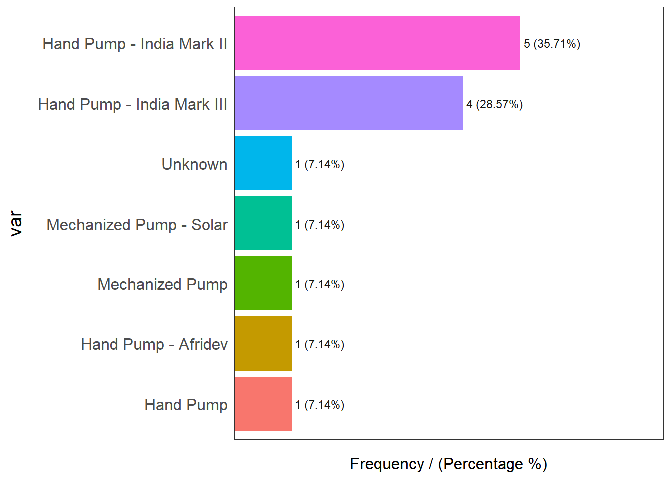
    freq(wp_joined3$water_tech_clean)

                             var frequency percentage cumulative_perc
    1  Hand Pump - India Mark II         5      35.71           35.71
    2 Hand Pump - India Mark III         4      28.57           64.28
    3                  Hand Pump         1       7.14           71.42
    4        Hand Pump - Afridev         1       7.14           78.56
    5            Mechanized Pump         1       7.14           85.70
    6    Mechanized Pump - Solar         1       7.14           92.84
    7                    Unknown         1       7.14          100.00
    Show the code
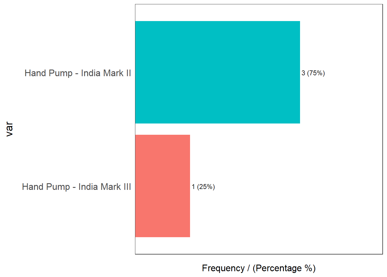
    freq(wp_joined3$water_tech_clean[wp_joined3$status == "Non-functional Technical breakdown"])

                             var frequency percentage cumulative_perc
    1  Hand Pump - India Mark II         3         75              75
    2 Hand Pump - India Mark III         1         25             100

    Remarks :

    Among the six (6) known water tech deployed to these 14 water points, two of these tech contributed to all these rehabilitated but non-functional due to technical breakdown.

    Show the code
    wtc_hPump3 <- wp_joined3 %>%
      filter(water_tech_clean %in%
               c("Hand Pump - India Mark II",
                 "Hand Pump - India Mark III",
                 "Hand Pump - India Mark III",
                 "Hand Pump",
                 "Hand Pump - Afridev"
                 ))
    wtc_iMii <- wtc_hPump3 %>%
      filter(water_tech_clean %in%
               "Hand Pump - India Mark II")
    
    wtc_iMiii <- wp_joined3 %>%
      filter(water_tech_clean %in%
               "Hand Pump - India Mark III")
    
    wp_nga3 <- wp_nga3 %>%
      mutate(`total_hPump` = lengths(
        st_intersects(bdy_nga, wtc_hPump3)
        )) %>%
      mutate(`total_iMii` = lengths(
        st_intersects(bdy_nga, wtc_iMii)
        )) %>%
      mutate(`total_iMiii` = lengths(
        st_intersects(bdy_nga, wtc_iMiii)
        )) %>%      
      mutate(`pct_iMii` = (`total_iMii`/`total_hPump`*100)) %>%
      mutate(`pct_iMiii` = (`total_iMiii`/`total_hPump`*100))