Show the code
pacman::p_load(sf, tmap, tidyverse)November 18, 2022
March 6, 2023
Choropleth mapping involves the symbolisation of enumeration units, such as countries, provinces, states, counties or census units, using area patterns or graduated colors.
E.g., use a choropleth map to portray the spatial distribution of aged population of <country>.
This exercise focuses on usage of tmap package to create choropleth map.
tmap :
qtm( )- to plot quick thematic map.
tm_shape( ) - specify the shape object.
tm_fill( ) / tm_polygons( ) - draw polygons.
tm_layout( ) - layout of cartographic map.
tm_borders( ) - draw polygon borders.
tm_compass( ) - map compass.
tm_scale_bar( ) - scale bar.
tm_grid( ) - draw coordinate grid / graticule lines.
tm_credits( ) - include credits text.
tmap_style( ) - set or get the default tmap style.
tmap_arrange( ) - create multiple stand-alone maps.
tm_facets( ) - define a group-by variable.
sf : st_read( ) - import shapefile as a simple feature data frame.
tidyverse, consists the following functions :
readr :
read_csv( ) - importing delimited text file.
tidyr :
mutate( ) - adds new variables and preserves existing ones.
mutate_at( ) - affects variables selected with a character vector or vars( ).
left_join( ) - join geographical data and attribute table.
filter( )
group_by( )
select( )
Master Plan 2014 Subzone Boundary (Web) : (i.e. MP14_SUBZONE_WEB_PL) in ESRI shapefile format from data.gov.sg
This is a geospatial data.
Consists of the geographical boundary of Singapore at the planning subzone level. The data is based on URA Master Plan 2014.
Singapore Residents by Planning Area / Subzone, Age Group, Sex and Type of Dwelling, June 2011-2020 : csv format (i.e. respopagesextod2011to2020.csv) from Department of Statistics, Singapore
This is an aspatial data file.
Although it does not contain any coordinates values, but it’s PA and SZ fields can be used as unique identifiers to geocode to MP14_SUBZONE_WEB_PL shapefile.
Reading layer `MP14_SUBZONE_WEB_PL' from data source
  `D:\jephOstan\ISSS624\data\geospatial' using driver `ESRI Shapefile'
Simple feature collection with 323 features and 15 fields
Geometry type: MULTIPOLYGON
Dimension:     XY
Bounding box:  xmin: 2667.538 ymin: 15748.72 xmax: 56396.44 ymax: 50256.33
Projected CRS: SVY21Rows: 323
Columns: 16
$ OBJECTID <int> 1, 2, 3, 4, 5, 6, 7, 8, 9, 10, 11, 12, …
$ SUBZONE_NO <int> 1, 1, 3, 8, 3, 7, 9, 2, 13, 7, 12, 6, 1…
$ SUBZONE_N <chr> "MARINA SOUTH", "PEARL'S HILL", "BOAT Q…
$ SUBZONE_C <chr> "MSSZ01", "OTSZ01", "SRSZ03", "BMSZ08",…
$ CA_IND <chr> "Y", "Y", "Y", "N", "N", "N", "N", "Y",…
$ PLN_AREA_N <chr> "MARINA SOUTH", "OUTRAM", "SINGAPORE RI…
$ PLN_AREA_C <chr> "MS", "OT", "SR", "BM", "BM", "BM", "BM…
$ REGION_N <chr> "CENTRAL REGION", "CENTRAL REGION", "CE…
$ REGION_C <chr> "CR", "CR", "CR", "CR", "CR", "CR", "CR…
$ INC_CRC <chr> "5ED7EB253F99252E", "8C7149B9EB32EEFC",…
$ FMEL_UPD_D <date> 2014-12-05, 2014-12-05, 2014-12-05, 20…
$ X_ADDR <dbl> 31595.84, 28679.06, 29654.96, 26782.83,…
$ Y_ADDR <dbl> 29220.19, 29782.05, 29974.66, 29933.77,…
$ SHAPE_Leng <dbl> 5267.381, 3506.107, 1740.926, 3313.625,…
$ SHAPE_Area <dbl> 1630379.3, 559816.2, 160807.5, 595428.9…
$ geometry <MULTIPOLYGON [m]> MULTIPOLYGON (((31495.56 3…Usage of the code chunk below :
sample( ) - base - to display only first 2 rows of data.
Simple feature collection with 2 features and 15 fields
Geometry type: MULTIPOLYGON
Dimension:     XY
Bounding box:  xmin: 28160.23 ymin: 28369.47 xmax: 32362.39 ymax: 30177.73
Projected CRS: SVY21
  OBJECTID SUBZONE_NO    SUBZONE_N SUBZONE_C CA_IND   PLN_AREA_N PLN_AREA_C
2        2          1 PEARL'S HILL    OTSZ01      Y       OUTRAM         OT
1        1          1 MARINA SOUTH    MSSZ01      Y MARINA SOUTH         MS
        REGION_N REGION_C          INC_CRC FMEL_UPD_D   X_ADDR   Y_ADDR
2 CENTRAL REGION       CR 8C7149B9EB32EEFC 2014-12-05 28679.06 29782.05
1 CENTRAL REGION       CR 5ED7EB253F99252E 2014-12-05 31595.84 29220.19
  SHAPE_Leng SHAPE_Area                       geometry
2   3506.107   559816.2 MULTIPOLYGON (((29092.28 30...
1 5267.381 1630379.3 MULTIPOLYGON (((31495.56 30...Rows: 984656 Columns: 7
── Column specification ────────────────────────────────────────────────────────
Delimiter: ","
chr (5): PA, SZ, AG, Sex, TOD
dbl (2): Pop, Time
ℹ Use `spec()` to retrieve the full column specification for this data.
ℹ Specify the column types or set `show_col_types = FALSE` to quiet this message.Prepare data table to plot thematic map. The variables are :
young : age group 0 to 4 until age groyup 20 to 24,
economy active : age group 25-29 until age group 60-64,
aged: age group 65 and above,
total : all age group, and
dependency : the ratio between young and aged against economy active group
Usage of the code chunk below :
pivot_wider( ) - - to display only first 2 rows of data.
pivot_wider(
  data,
  id_cols = NULL, id_expand = FALSE, names_from = name, names_prefix = "",
  names_sep = "_", names_glue = NULL, names_sort = FALSE, names_vary = "fastest",
  names_expand = FALSE, names_repair = "check_unique", values_from = value,
  values_fill = NULL, values_fn = NULL, unused_fn = NULL, ...
)

arguments :

* data = A data frame to pivot.

* id_cols = A set of columns that uniquely identifies each observation.
>> Defaults to all columns in data except for the columns specified in names_from and values_from.
>> Typically used when have redundant variables, i.e. variables whose values are perfectly correlated with existing variables.

* id_expand = Should the values in the id_cols columns be expanded by expand() before pivoting?
>> This results in more rows, the output will contain a complete expansion of all possible values in id_cols.
>> Implicit factor levels that aren't represented in the data will become explicit.
>> Additionally, the row values corresponding to the expanded id_cols will be sorted.

* names_from, values_from = A pair of arguments describing which column (or columns) to get the name of the output column (names_from), and which column (or columns) to get the cell values from (values_from).
>> If values_from contains multiple values, the value will be added to the front of the output column.
more arguments for pivot_wider() …
mutate(.data, ...,
  .keep = c("all", "used", "unused", "none"),
  .before = NULL,
  .after = NULL
)

arguments :

* data = A data frame, data frame extension (e.g. a tibble), or a lazy data frame (e.g. from dbplyr or dtplyr)

* ... = Name-value pairs. The name gives the name of the column in the output.

* keep = Control which columns from .data are retained in the output.
>> Grouping columns and columns created by ... are aways kept.
"all" retains all columns from .data. This is the default.

"used" retains only the columns used in ... to create new columns. This is useful for checking your work, as it displays inputs and outputs side-by-side.

"unused" retains only the columns not used in ... to create new columns. This is useful if you generate new columns, but no longer need the columns used to generate them.

"none" doesn't retain any extra columns from .data. Only the grouping variables and columns created by ... are kept.

* .before, .after = Optionally, control where new columns should appear (the default is to add to the right hand side).`summarise()` has grouped output by 'PA', 'SZ'. You can override using the
`.groups` argument.popdata2020 <- popdata %>%
filter(Time == 2020) %>%
group_by(PA, SZ, AG) %>%
summarise(`POP` = sum(`Pop`)) %>%
ungroup()%>%
pivot_wider(names_from=AG,
values_from=POP) %>%
mutate(YOUNG = rowSums(.[3:6])
+rowSums(.[12])) %>%
mutate(`ECONOMY ACTIVE` = rowSums(.[7:11])+
rowSums(.[13:15]))%>%
mutate(`AGED`=rowSums(.[16:21])) %>%
mutate(`TOTAL`=rowSums(.[3:21])) %>%
mutate(`DEPENDENCY` = (`YOUNG` + `AGED`)
/`ECONOMY ACTIVE`) %>%
select(`PA`, `SZ`, `YOUNG`,
`ECONOMY ACTIVE`, `AGED`,
`TOTAL`, `DEPENDENCY`)`summarise()` has grouped output by 'PA', 'SZ'. You can override using the
`.groups` argument.![]() Useful mutate functions :
Useful mutate functions :
+, -, log( ), etc., for their usual mathematical meanings
lead( ), lag( )
dense_rank( ), min_rank( ), percent_rank( ), row_number( ), cume_dist( ), ntile( )
cumsum( ), cummean( ), cummin( ), cummax( ), cumany( ), cumall( )
na_if( ), coalesce( )
if_else( ), recode( ), case_when( )
The 3 scoped variants of mutate( ) to transform multiple variables :
_all affects every variable
_at affects variables selected with a character vector or vars()
_if affects variables selected with a predicate function.
mutate_at(.tbl, .vars, .funs, ..., .cols = NULL)

arguments :

* .tbl = A tbl object.

* .funs = A function, a quosure style lambda ~ fun(.) or a list of either form.
>> can be a named or unnamed list. If a function is unnamed and the name cannot be derived automatically, a name of the form "fn#" is used.

* ... = Additional arguments for the function calls in .funs. These are evaluated only once, with tidy dots support.

*.vars = A list of columns generated by vars(), a character vector of column names, a numeric vector of column positions, or NULL.

* .cols = This argument has been renamed to .vars to fit dplyr's terminology and is deprecated.
[Before the georelational join, convert the values in PA and SZ fields to uppercase.]{style=“color:#9e6024”}
Warning: `funs()` was deprecated in dplyr 0.8.0.
ℹ Please use a list of either functions or lambdas:

# Simple named list: list(mean = mean, median = median)

# Auto named with `tibble::lst()`: tibble::lst(mean, median)

# Using lambdas list(~ mean(., trim = .2), ~ median(., na.rm = TRUE))
[To ensure the output is a simple features data frame, join data and attribute table using planning subzone name e.g. SUBZONE_N and SZ as the common identifier.]{style=“color:#9e6024”}
write_rds(
  x, file, compress = c("none", "gz", "bz2", "xz"), version = 2,
  refhook = NULL, text = FALSE, path = deprecated(), ...
)

arguments :

* file = The file path to read from/write to.

* refhook = A function to handle reference objects.

* x = R object to write to serialise.

* compress = Compression method to use: "none", "gz" ,"bz", or "xz".

* version = Serialization format version to be used. The default value is 2 as it's compatible for R versions prior to 3.5.0. See base::saveRDS() for more details.

* text = If TRUE a text representation is used, otherwise a binary representation is used.

* path = [Deprecated] Use the file argument instead.

* ... = Additional arguments to connection function. For example, control the space-time trade-off of different compression methods with compression. See connections() for more details.2 tmap approaches to prepare thematic map :
plot thematic map quickly using qtm( ).
plot highly customisable thematic map.
qtm(
  shp, fill = NA, symbols.size = NULL, symbols.col = NULL, symbols.shape = NULL,
  dots.col = NULL, text = NULL, text.size = 1, text.col = NA, lines.lwd = NULL,
  lines.col = NULL, raster = NA, borders = NA, by = NULL, scale = NA, title = NA,
  projection = NULL, bbox = NULL, basemaps = NA, overlays = NA, style = NULL,
  format = NULL, ...
)

arguments :

* shp = One of -
>> shape object, which is an object from a class defined by the sf or stars package. Objects from the packages sp and raster are also supported, but discouraged.

>> Not specified, i.e. qtm() is executed. In this case a plain interactive map is shown.

>> A OSM search string, e.g. qtm("Amsterdam"). In this case a plain interactive map is shown positioned according to the results of the search query (from OpenStreetMap nominatim)


* fill = either a color to fill the polygons, or name of the data variable in shp to draw a choropleth.
>> Only applicable when shp contains polygons.
>> Set fill = NULL to draw only polygon borders. See also argument borders.Arguments for the following function :
argument :

* style = method to process the color scale when col is a numeric variable.

>> Discrete gradient options are "cat", "fixed", "sd", "equal", "pretty", "quantile", "kmeans", "hclust", "bclust", "fisher", "jenks", "dpih", "headtails", and "log10_pretty".

>> A numeric variable is processed as a categorical variable when using "cat", i.e. each unique value will correspond to a distinct category.

>> For the other discrete gradient options (except "log10_pretty"), see the details in classIntervals (extra arguments can be passed on via style.args).

>> Continuous gradient options are "cont", "order", and "log10".

>> The numeric variable can be either regarded as a continuous variable or a count (integer) variable.

* legend.hist = logical that determines whether a histogram is shown.

* legend.hist.z = index value that determines the position of the histogram legend element.

* legend.is.portrait = logical that determines whether the legend is in portrait mode (TRUE) or landscape (FALSE).
tm_layout( ) - layout of cartographic map.
tm_borders( ) - draw polygon borders.
tm_borders(col = "grey40", lwd = 1, lty = "solid", alpha = NA)

argument :

* alpha = transparency number between 0 (totally transparent) and 1 (not transparent).
>> By default, the alpha value of the col is used (normally 1).

* col = border colour.

* lwd = border line width.

* lty = border line type.
tm_compass(north = 0, type = NA, text.size = 0.8, size = NA,
  show.labels = 1, cardinal.directions = c("N", "E", "S", "W"),
  text.color = NA, color.dark = NA, color.light = NA, lwd = 1,
  position = NA, bg.color = NA, bg.alpha = NA, just = NA,
  fontsize = NULL
)

arguments :

* type = compass type : "arrow", "4star", "8star", "radar", "rose". >> The default is controlled by tm_layout (which uses "arrow" for the default style)

* size = size of the compass in number of text lines.
>> The default values depend on the type: for "arrow" it is 2, for "4star" and "8star" it is 4, and for "radar" and "rose" it is 6.
tm_scale_bar( ) - scale bar.
tm_grid( ) - draw coordinate grid / graticule lines.
tm_grid(x = NA, y = NA, n.x = NA, n.y = NA, projection = NA,
  col = NA, lwd = 1, alpha = NA, labels.size = 0.6, labels.col = NA,
  labels.rot = c(0, 0), labels.format = list(big.mark = ","),
  labels.margin.x = 0, labels.margin.y = 0, labels.inside.frame = TRUE)

argument :

* alpha = transparency of the grid lines. Number between 0 and 1.
>> By default, the alpha transparency of col is taken.
tm_credits(text, size = 0.7, col = NA, alpha = NA, align = "left",
  bg.color = NA, bg.alpha = NA, fontface = NA, fontfamily = NA,
  position = NA, width = NA, just = NA
)

argument :
* position = position of the text. Vector of two values, specifying the x and y coordinates.

>> first value can be "left", "LEFT", "center", "right", or "RIGHT" >> second value can be "top", "TOP", "center", "bottom", or "BOTTOM"
>> or this vector contains two numeric values between 0 and 1 that specifies the x and y value of the center of the text.
>> The uppercase values correspond to the position without margins (so tighter to the frame).tm_shape(mpsz_pop2020)+
tm_fill("DEPENDENCY",
style = "quantile",
palette = "Blues",
title = "Dependency ratio") +
tm_layout(main.title = "Distribution of Dependency Ratio by planning subzone",
main.title.position = "center",
main.title.size = 1.2,
legend.height = 0.45,
legend.width = 0.35,
frame = TRUE,
asp = 0) +
tm_borders(alpha = 0.5) +
tm_compass(type="8star", size = 2) +
tm_scale_bar() +
tm_grid(alpha =0.2) +
tm_credits("Source: Planning Sub-zone boundary from Urban Redevelopment Authorithy (URA)\n and Population data from Department of Statistics DOS",
position = c("left", "bottom"))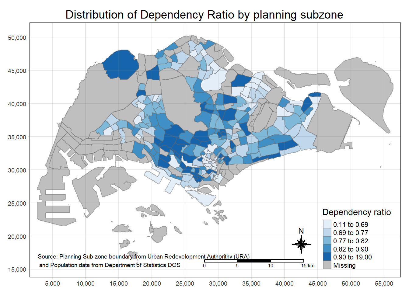
Following are the steps to reproduce above map.
Basic building block of tmap
The default interval binning used to draw the choropleth map is called “pretty”. A detailed discussion of the data classification methods supported by tmap will be provided in sub-section 4.3.
The default colour scheme used is YlOrRd of ColorBrewer. You will learn more about the color scheme in sub-section 4.4.
By default, Missing value will be shaded in grey.
tm_polygons( ) is a wraper of tm_fill( ) & tm_border( ).
tm_fill( ) shades the polygons by using the default colour scheme.
tm_borders( ) adds the borders of the shapefile onto the choropleth map.
tmap provides a total ten data classification methods, namely: fixed, sd, equal, pretty (default), quantile, kmeans, hclust, bclust, fisher, and jenks.
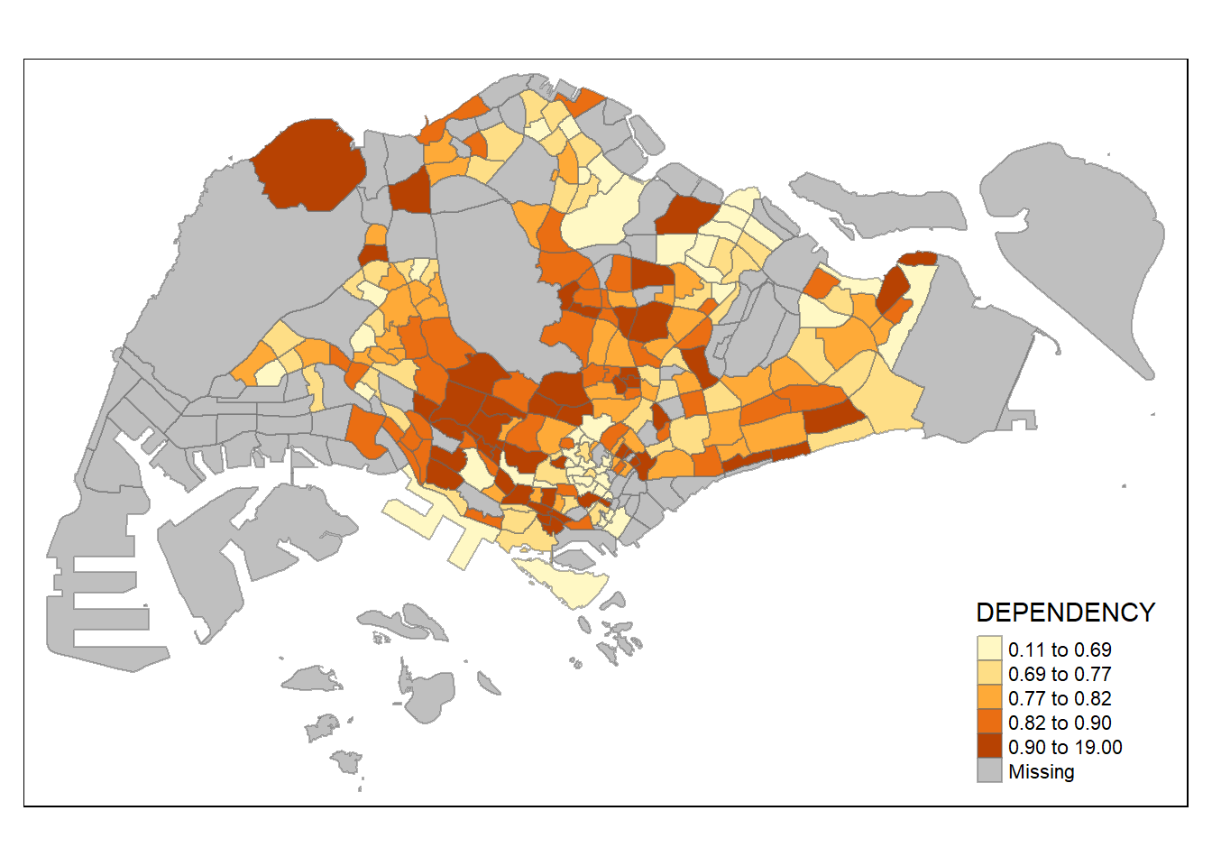
DIY: Preparing choropleth maps by using similar classification method but with different numbers of classes (i.e. 2, 6, 10, 20). Compare the output maps, what observation can you draw?
Tmap breaks require a minimum and maximum.
In order to end up with n categories, n+1 elements must be specified in the breaks option (the values must be in increasing order).
Before setting the break points, use summary( ) to compute descriptive statistics of the “DEPENDENCY” variable.
   Min. 1st Qu.  Median    Mean 3rd Qu.    Max.    NA's
 0.1111  0.7147  0.7866  0.8585  0.8763 19.0000      92
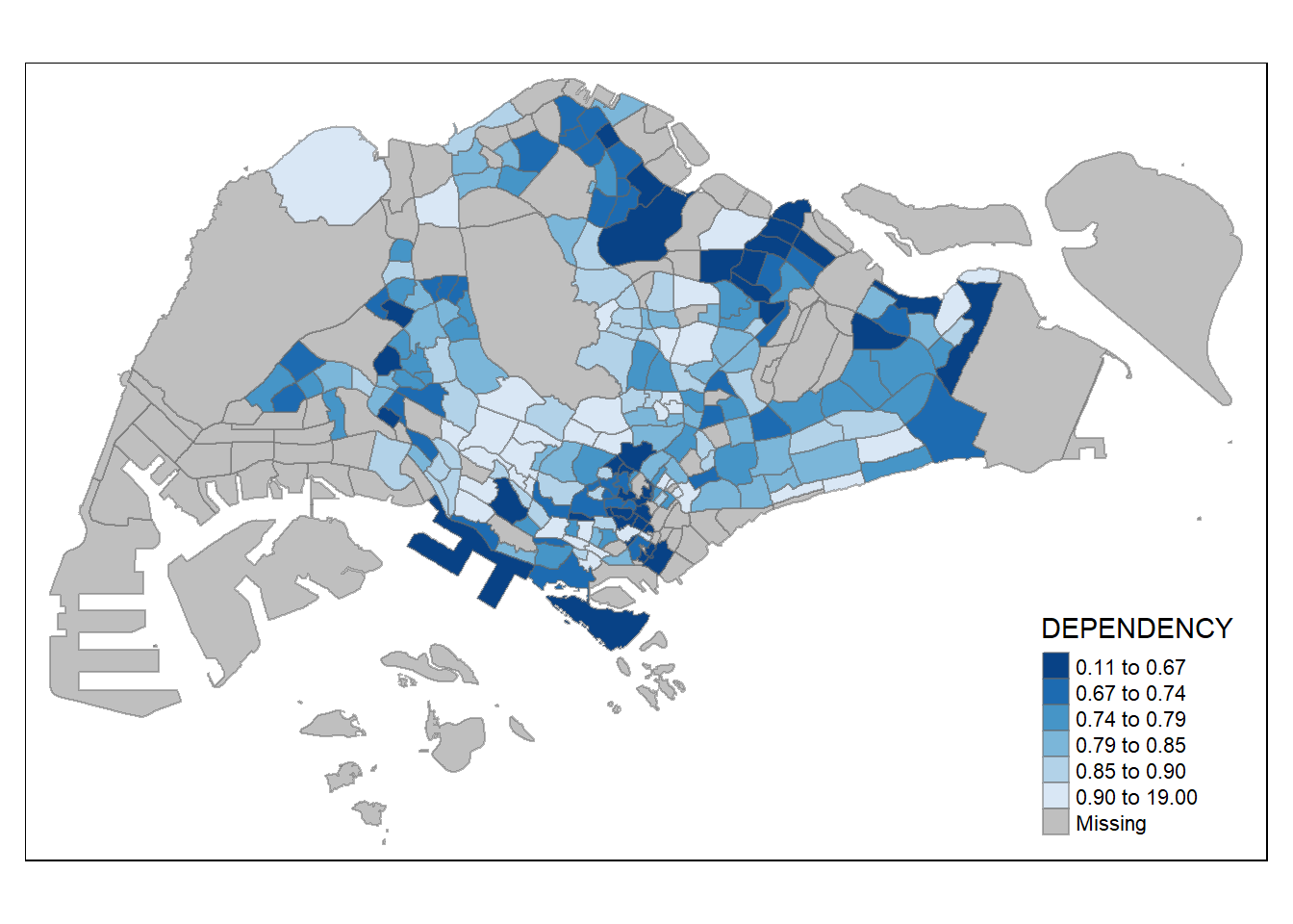
Set break point at 0.60, 0.70, 0.80, and 0.90.
Need to include a minimum and maximum, which set at 0 and 100.
Breaks vector is thus c(0, 0.60, 0.70, 0.80, 0.90, 1.00)
Warning: Values have found that are higher than the highest break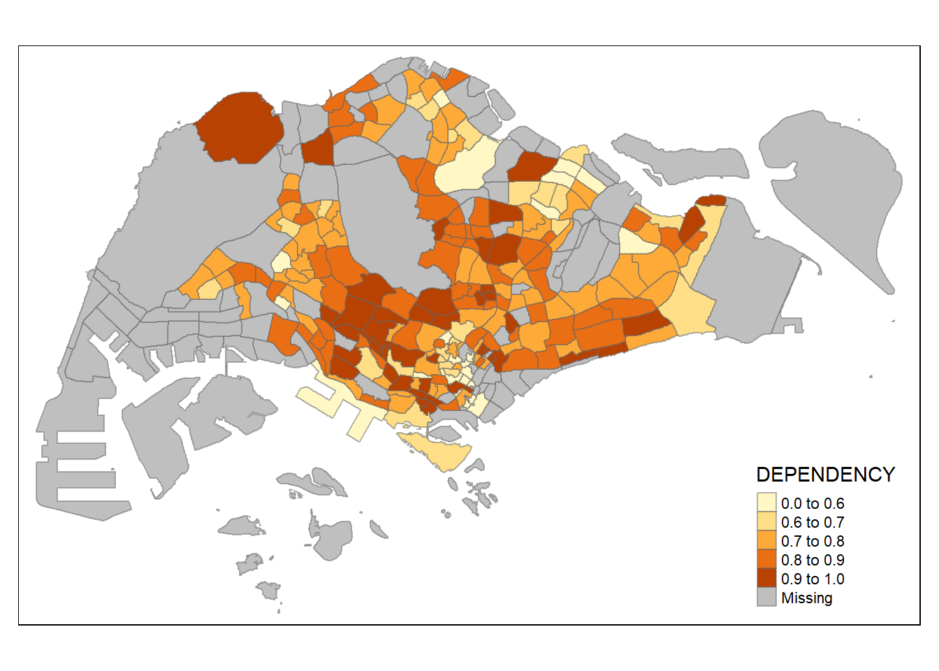
quick reference for ColorBrewer 2.0 colour options
use palette argument in tm_fill( )
without “-” prefix, darker shade = higher value
with “-” prefix to reverse colour scheme, darker shade = smaller value
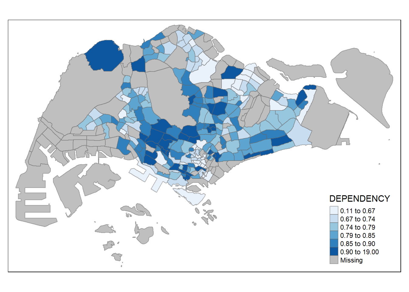
tm_shape(mpsz_pop2020)+
  tm_fill("DEPENDENCY",
          style = "jenks",
          palette = "Blues",
          legend.hist = TRUE,
          legend.is.portrait = TRUE,
          legend.hist.z = 0.1) +
  tm_layout(main.title = "Distribution of Dependency Ratio by planning subzone \n(Jenks classification)",
            main.title.position = "center",
            main.title.size = 1,
            legend.height = 0.45,
            legend.width = 0.35,
            legend.outside = FALSE,
            legend.position = c("right", "bottom"),
            frame = FALSE) +
  tm_borders(alpha = 0.5)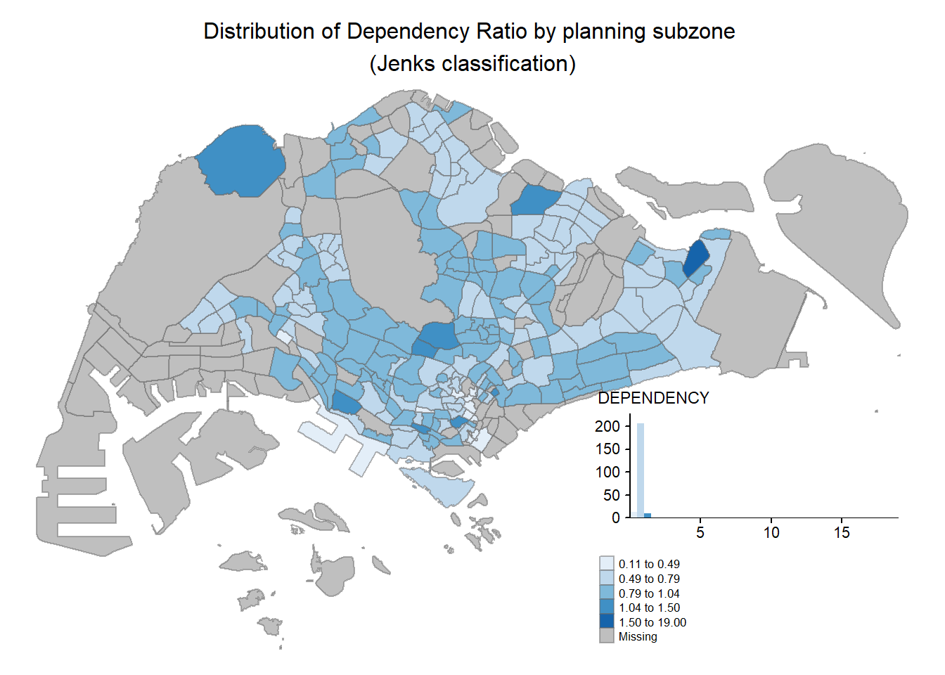
use tmap_style( ) function.
the default style is “white”.
Other map furniture such as compass, scale bar, grid lines, etc.
tm_shape(mpsz_pop2020)+
  tm_fill("DEPENDENCY",
          style = "quantile",
          palette = "Blues",
          title = "No. of persons") +
  tm_layout(main.title = "Distribution of Dependency Ratio \nby planning subzone",
            main.title.position = "center",
            main.title.size = 1.2,
            legend.height = 0.45,
            legend.width = 0.35,
            frame = TRUE) +
  tm_borders(alpha = 0.5) +
  tm_compass(type="8star", size = 2) +
  tm_scale_bar(width = 0.15) +
  tm_grid(lwd = 0.1, alpha = 0.2) +
  tm_credits("Source: Planning Sub-zone boundary from Urban Redevelopment Authorithy (URA)\n and Population data from Department of Statistics DOS",
             position = c("left", "bottom"))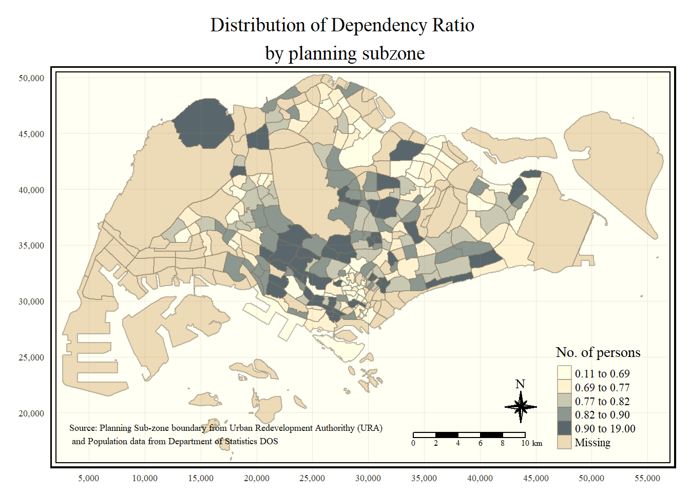
Small multiple maps (smm), also referred to as facet maps, are composed of many maps arrange side-by-side, and sometimes stacked vertically.
In tmap, can be plotted in 3 ways:
by assigning multiple values to at least one of the asthetic arguments,
by defining a group-by variable in tm_facets( ), and
by creating multiple stand-alone maps with tmap_arrange( ).
tmap style set to "white"other available styles are: "gray", "natural", "cobalt", "col_blind", "albatross", "beaver", "bw", "classic", "watercolor" 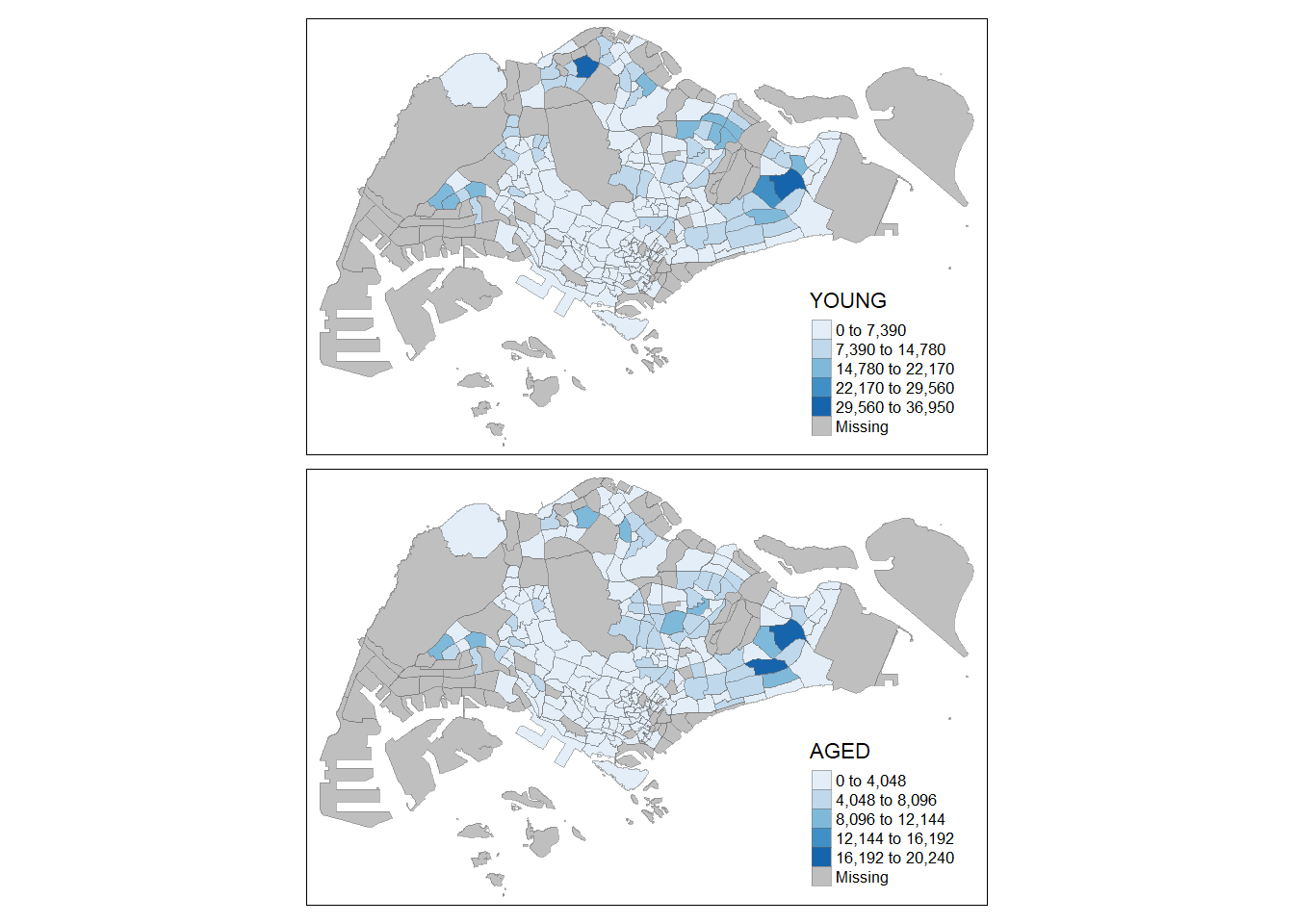
Warning: The argument drop.shapes has been renamed to drop.units, and is
therefore deprecated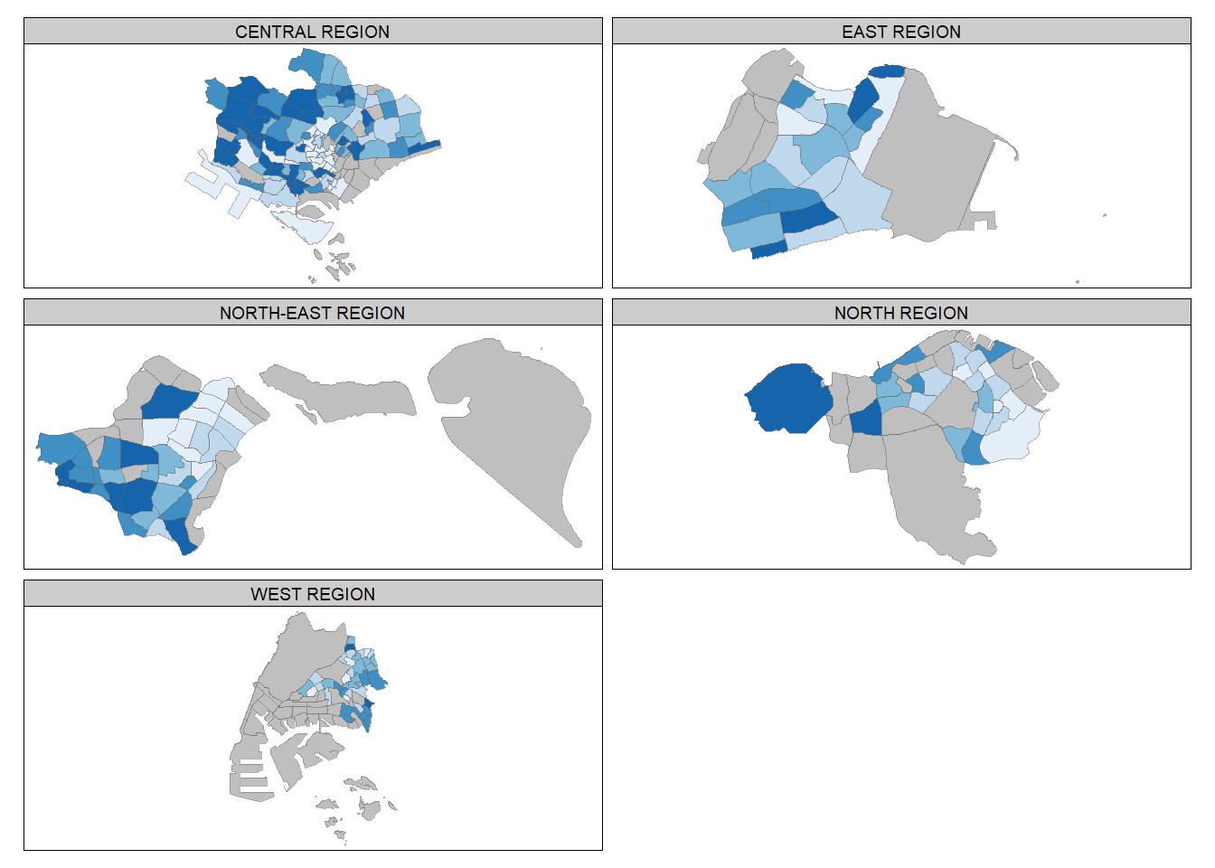
tm_shape(mpsz_pop2020[mpsz_pop2020$REGION_N=="CENTRAL REGION", ])+
  tm_fill("DEPENDENCY",
          style = "quantile",
          palette = "Blues",
          legend.hist = TRUE,
          legend.is.portrait = TRUE,
          legend.hist.z = 0.1) +
  tm_layout(legend.outside = TRUE,
            legend.height = 0.45,
            legend.width = 5.0,
            legend.position = c("right", "bottom"),
            frame = FALSE) +
  tm_borders(alpha = 0.5)
Warning in pre_process_gt(x, interactive = interactive, orig_crs =
gm$shape.orig_crs): legend.width controls the width of the legend within a map.
Please use legend.outside.size to control the width of the outside legend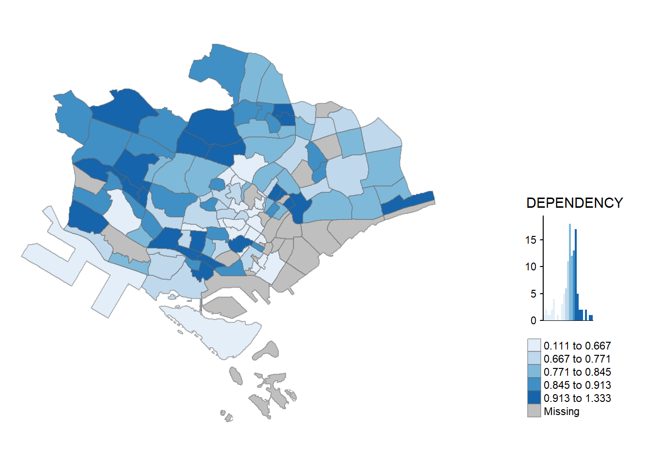
Datacamp. Writing.rds files. https://campus.datacamp.com/courses/reading-data-into-r-with-readr/importing-data-with-readr?ex=7
Dplyr.tidyverse.org. Mutate multiple columns. https://dplyr.tidyverse.org/reference/mutate_all.html
qtm: Quick thematic map plot. https://www.rdocumentation.org/packages/tmap/versions/3.3-3/topics/qtm
r4gdsa.netlify.app. https://r4gdsa.netlify.app/chap02.html#data-preparation
Rdocumentation.org. tm_shape: Specify the shape object. https://www.rdocumentation.org/packages/tmap/versions/3.3-3/topics/tm_shape
Tidyr.tidyverse.org. Pivot data from long to wide. https://tidyr.tidyverse.org/reference/pivot_wider.html