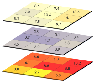
Geographically Weighted Logistic Regression (GWLR)

#PERSONAL NOTES

1. OVERVIEW

Key Focuses

1. Understand the differences between binary and continuous outcomes.
2. Understand the basic concepts and methods of logistic regression models.
3. Interpret the model and analysis results accurately.
4. Compare and evaluate predictive models generated using logistic regression.

Key Questions :

• How do I tell if my model is good?

• How do I tell if the explanatory variable helping my model?

• How do I tell if my model is providing reasonable prediction?

2. DATA TYPE

Various types of data :

• Branch (Categorical: Toronto, Montreal, Seattle, etc.)

• Attrition (Binary: Stay, Churn)

• Promotion (Binary: Promoted, Not Promoted)

• Sales Plan (Continuous, this is how much an employee must sell in that month)

But, in the context of spatial data, there are two (2) primary types¹ :

¹ GISGeography. (2022, May 28 May). Vector vs Raster: What’s the Difference Between GIS Spatial Data Types? https://gisgeography.com/spatial-data-types-vector-raster/

• Vector data is comprised of vertices and paths.

  • 3 basic symbol types :

    • points = XY coordinates with a spatial reference frame.

    • lines = Each dot representing a vertex. Lines connect each vertex in a set order to be a vector line.

    • polygons (areas) = vector polygon formed when joining a set of vertices in a particular order and closing it.

Raster data consists of 2 categories :

• Discrete Raster has a distinct theme or category.

  • Each land cover cell is definable.

  • It can be discreetly defined where the class begins and ends.

  • Usually consists of integers to present classes. E.g. value 1 = urban areas, 2 = forest, etc.

• Continuous Raster (non-discrete) are grid cells with gradually changing data.

  • E.g. elevation, temperature, aerial photograph, etc.

  • A continuous raster surface can be derived from a fixed registration point.

    -- Digital elevation models use sea level as a registration point.

    -- Cell values for aspect map² have fixed directions such as north, east, south, or west.

² GISGeography. (2022, November 9). What is an Aspect Map? https://gisgeography.com/aspect-map/

Continuous data is poorly stored and displayed as vectors. To display continuous data as a vector would require substantial generalisation. Although topology is useful for vector data, it is often processing intensive.

Generally, quantitative analysis is intuitive with discrete or continuous raster. However, it can be potentially huge at the cost of processing speed and data storage.

Example 1

Whether a customer churns, (y = 1) or not churns (y = 0) after signed up a mobile service contract.

• probability (p) depends on x.
• x is the explanatory variable (either categorical (discrete) or quantitative), such as :
  • account age
  • current billing amount
  • average days delinquent

3. LOGISTIC REGRESSION MODELS

Logistic regression model can be used as :

• explanatory model

• predictive model

The logistic model (or logit model)³ is a statistical model that models the probability of an event taking place by having the log-odds for the event be a linear combination of one or more independent variables.

³ Wikipedia. (n.d.). Logistic regression. https://en.wikipedia.org/wiki/Logistic_regression

In regression analysis, logistic regression (or logit regression) estimates the parameters of a logistic model (the coefficients in the linear combination).

Revision Note

Regression analysis⁴ is a set of statistical processes for estimating the relationships between :

⁴ Wikipedia. (n.a.). Regression analysis. https://en.wikipedia.org/wiki/Regression_analysis

• a dependent variable (often called the ‘outcome’ or ‘response’ variable, or a ‘label’ in machine learning parlance), and

• one or more independent variables (often called ‘predictors’, ‘covariates’, ‘explanatory variables’ or ‘features’)

In Binary Logistic Regression, usually consists :

• A single binary dependent variable, coded by an indicator variable, where the two values are labelled “0” and “1”.

• The independent variables can each be a binary variable (two classes coded by an indicator variable) or a continuous variable (any real value).

  • The corresponding probability of the value labelled “1” can vary between 0 and 1.

  • Logistic function converts log-odds to probability.

    -- Logistic functions are used in logistic regression to model how the probability p of an event may be affected by one or more explanatory variables.

  • The unit of measurement for the log-odds scale is called a logit, from logistic unit.

3.1 Linear Regression

3.1.1 Assumptions of Linear Regression

When the value of a variable is a binary response, the linear regression assumptions are not valid based on the following :

• the relationship between the independent variable and predictor variable is not linear.

• the error terms are :

  • heteroscedastic

  • not normally distributed

Violated Linear Regression Assumptions

If proceeding in light of these violations, the results would be :

• the predicted probabilities can be greater than 1 or less than 0.

• the magnitude of the effects of independent variables may be greatly underestimated.

3.2 Logistic Regression

A simple linear regression modeled the mean μ of the response variable y as a linear function of the explanatory variable : 𝜇 = 𝛽0 + 𝛽1𝑥.

A logistic regression would model the mean of the response variable p in terms of an explanatory variable x.

• BUT, this is not a good model when relating p and x through the equation 𝑝 = 𝛽0 + 𝛽1𝑥.

• As long as 𝛽0 ≠ 0, extreme values of x will give values of 𝛽0 + 𝛽1𝑥 that is inconsistent with the fact that 0 ≤ p ≤ 1.

3.2.1 Assumptions of Logistic Regression

• Logistic regression does not assume a linear relationship between the dependent and independent variables.

• For binary logistic regression, the dependent variable must be a dichotomy (2 categories).

• The independent variables need not be interval, normally distributed, linearly related, nor of equal variance within each group.

• The categories (groups) must be mutually exclusive and exhaustive.

• A case can only be in one group, and every case must be a member of one of the groups.

Unlike linear regression, larger samples are needed for logistic regression because maximum likelihood coefficients are large sample estimates.

Minimum of 50 observations / cases per indepdent variables / predictors is recommended.

Logistic Regression Solution :: Log Odds

Transform the odds to get odds ratio, 𝑝 / 1−𝑝

note : logistic regressions work with odds rather than proportions.

• Model the log odds as a linear function of the explanatory variable.

• The slope in a logistic regression model = the difference between the log(ODDS) for churn and the log(ODDS) for not churn.

• Logistic distribution constrains the estimated probability between 0 and 1, via :

  𝑝 = 1 / 1+𝑒−(𝛽0+𝛽1𝑥)

  • 𝛽0 + 𝛽1𝑥 = 0 , then p = .50

  • 𝛽0 + 𝛽1𝑥 gets really big, p approaches 1

  • 𝛽0 + 𝛽1𝑥 gets really small, p approaches 0

3.2.1 Odds Definition

Odds are the ratio of the proportions for the two possible outcomes.

Odds(event) = P(event) / 1-P(event)

Example 2

Total customers = 13,196

Churn = 1,091

Sample proportion, p^ = 1,091 / 13,196 = 0.0827

Odds = 0.0827 / 0.9173 = 0.0902

Interpretation :

The odds that a customer is going to churn as 9 to 100.

3.2.2 Interpret Simple Logistic Regression

Example 3

simple logistic regression, ln (𝑃 / 1 − 𝑝) = 0.5954 + −0.0255(account_age)

For account_age = 20,

ln (𝑃 / 1 − 𝑃) = 0.5954 + −0.0255(20) = 0.0854

𝑒0.0854 / (1 + 𝑒0.0854) = 0.5213

note :

• For every 1 month increase in account_age, the logit of the probability of a churn decrease by 0.0255.

• Given account_age of a customer is 20, the log-odds = 0.0854

• Probability of Churn (also known as probability of log-odds) = 0.5213

Interpretation :

A customer with 20 months account_age has an average of 0.5213 chance that she/he will churn.

3.3 Difference of Multiple Logistic Regression & Linear Regression

Instead of using a least-squared deviations criterion for the best fit, it uses a maximum likelihood method, which maximizes the probability of getting the observed results given the fitted regression coefficients.

A consequence is that the goodness of fit and overall significance statistics used in logistic regression differ from those used in linear regression.

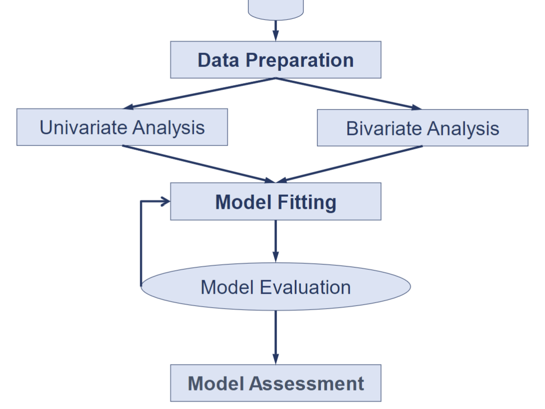
3.3.1 Workflow Diagram :: Logistic Regression Modelling

3.3.2.1 Univariate Analysis

Check for outliers and determine the distribution of each predictor variable.

Determine which dummy variables to create as a predictor variables.

compare “No Churn” value among variables

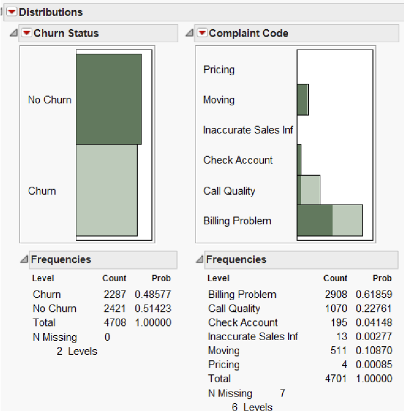
• E.g. the figure above shows that when “No churn” cases are strongly related to “Moving” and “Check Account” under the “Complain Code” variable.

  • Consider combining “Moving” and “Check Account” to form a group.

3.3.2.2 Bivariate Analysis

Similar to multiple linear regression, the logistic regression model is sensitive to multicollinearity.

• Multicollinearity occurs when some of the predictors are highly correlated.

4. MODEL PERFORMANCE EVALUATION

4.1 Methods to Evaluate Logistic Regression Model

There are several statistics which can be used for comparing alternative models or evaluating the performance of a logistic regression model :

• Whole model test
• Fit statistics
• Assessing individual parameters

4.1.1 Whole Model Test

Testing :

𝐻0 : The logistic model is NOT useful.

𝐻1 : The logistic model is useful.

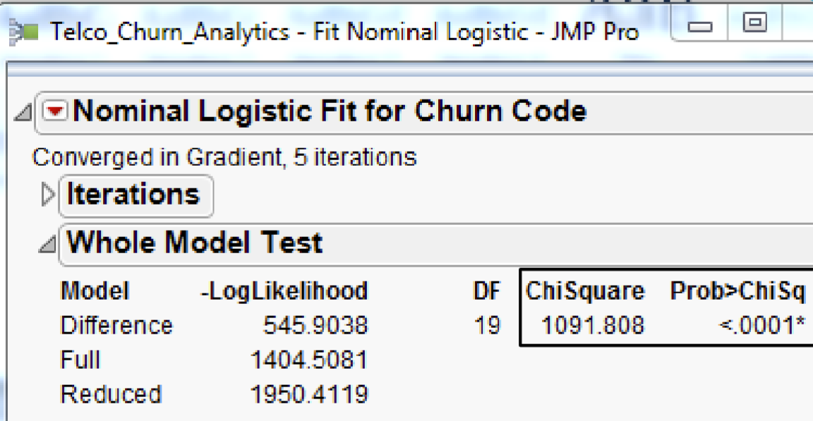
The test is analogous to the Analysis of Variance table for continuous responses.

The negative log-likelihood corresponds to the sums of squares, and the Chi-square test corresponds to the F-test.

Decision :

Reject 𝐻0 if the Chi Square is large and the 𝑝 value is smaller than the critical value (i.e. 0.05, or 0.01, 0.001, 0.0001).

• The 𝑝-value < 0.0001* indicates that the logistic model is useful to explain the ODDS(churn).

• In other words, the overall model is significant at the .0001 level according to the Model chi-square statistic.

4.1.2 Lack of Fit Test (Goodness of Fit)

Testing :

𝐻0 : The model is adequate.

𝐻1 : The model is inadequate, i.e. there is lack of fit.

Decision :

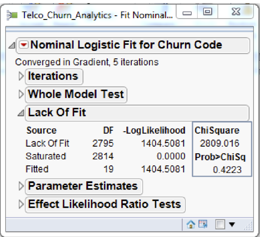
Reject 𝐻0 if the Chi Square statistics is large and the 𝑝 value is smaller than the critical value (i.e. 0.05, or 0.01, 0.001, 0.0001).

The above figure shows that the Lack of Fit Chi-square is not significant (Prob > ChiSq = 0.4223) and supports the conclusion that there is little to be gained by introducing additional variables.

4.1.2.1 Likelihood-ratio Test (LRT, Wilks Test)

The likelihood-ratio test assesses the goodness of fit of two competing statistical models based on the ratio of their likelihoods⁵, specifically one found by maximisation over the entire parameter space and another found after imposing some constraint.

⁵ Wikipedia. (n.d.). Likelihood-ratio test. https://en.wikipedia.org/wiki/Likelihood-ratio_test

LRT tests are computed iteratively and can be computationally intensive for some models. So, historically Wald’s tests had been used more often.

The Effect Likelihood Ratio Tests report above show that both predictor variables Avg Days Delinquent and Account Age are significant at p < 0.0001 and predictor Condition of Current Handset is not significant p = 0.3181.

Note : LRT are more reliable than Wald’s tests, so use LRT when possible.

4.1.3 Assessing Individual Parameters

Testing :

𝐻0 : 𝛽1 = 0

𝐻1 : 𝛽1 ≠ 0

Test statistics, 𝑍 = 𝑏1 / 𝑆𝐸_𝑏1

Statistical inference for multiple logistic regression is similar to statistical inference for multiple linear regression.

• Calculate estimates of the model parameters and standard errors.

• Confidence intervals are formed in the usual way but use standard normal z∗-values rather than critical values from the t distributions.

• The ratio of the estimate to the standard error is the basis for hypothesis tests.

• Often the test statistics are given as the squares of these ratios.

  • In this case, the P-values are obtained from the chi-square distributions with 1 degree of freedom.

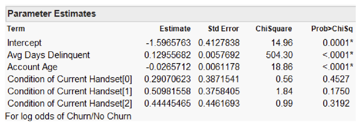
Output from some statistical software reports the significance test results in terms of chi-square statistic, i.e. square of the z statistic / Wald statistic.

𝑋² = 𝑥²

• When the null hypothesis is true, it has a distribution that is approximately a 𝑥² distribution with 1 degree of freedom, and the P-value is calculated as P ( 𝑥² ≥ 𝑋² ).

• Because the square of a standard normal random variable has a 𝑥² distribution with 1 degree of freedom, the 𝑧 statistic and the chi-square statistic give the same results for statistical inference.

  • The Parameter Estimates report reveals that not all predictor variables are significant.

  • In fact, only Avg Days Delinquent and Account Age with p-values < 0.0001.

  • The Condition of Current Handset is not significant.

4.2 Accuracy of Predictive Modelling

4.2.1 Contigency Table / Error Table / Confusion Matrix

In binomial logistic regression, the classification table is a 2 x 2 table that contains the observed and predicted model results.

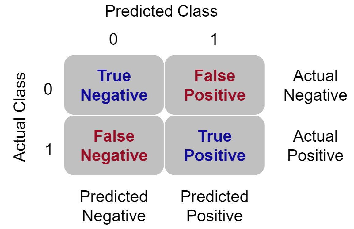
The contingency table has 4 data cells :

1. Actual 0 Predicted 0 – The number of cases predicted and observed as 0.

   • The records in this cell are referred to as true negatives.

   • The model classification was correct for these records.

2. Actual 0 Predicted 1 – The number of cases predicted as 1 yet observed as 0.

   • The records in this cell are referred to as false positives.

   • The model classification was incorrect for these records.

3. Actual 1 Predicted 1 – The number of cases predicted and observed as 1.

   • The records in this cell are referred to as true positives.

   • The model classification was correct for these records.

4. Actual 1 Predicted 0 – The number of cases predicted as 0 yet observed as 1.

   • The records in this cell are referred to as false negatives.

   • The model classification was incorrect for these records.

The model classifies each data record based on :

• The computed probability is between 0 and 1.

• The threshold / cut value = the minimal probability value to classify as 0 or 1.

  • The default “cut value” is 0.5. When a value is greater than 0.5, it will be classified as 1.

Different fields of applications has different tolerable rates of false positives and false negatives.

4.2.2 Assess Model Performance :: Misclassification Rate

Classification Table / Contigency Table is used to assess the overall performance of a logistic regression model.

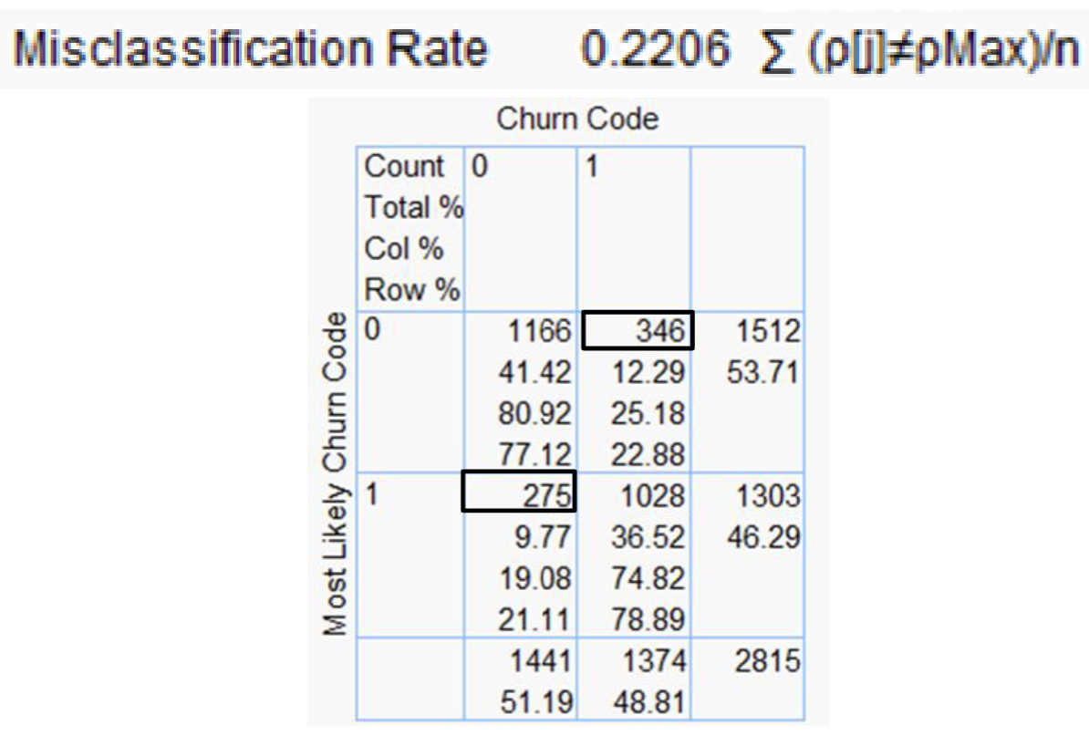
• The classification table above shows that there are 346 false negative and 275 false positive. The overall misclassification error is 22.06%, i.e. ( 346 + 275 ) / 2815 ).

• According to the Misclassification Rate measure, the model predicts 77.94% of the churn cases correctly.

4.2.2.1 Contingency Analysis

1. Overall Accuracy

   Refers to the correctly classified observations divided by the total number of observations.

   • This statistics is not a particularly useful measure because it gives equal weight to all components.

overall_accuracy = ( 𝑻𝑷 + 𝑻𝑵 ) / ( 𝑻𝑷 + 𝑭𝑷 + 𝑭𝑵 + 𝑻𝑵 )

2. Sensitivity refers to the true positive rate.

sensitivty = ( 𝑻𝑷 ) / ( 𝑻𝑷 + 𝑭𝑵 )

3. Specificity refers to the true negative rate.

specificity = ( 𝑻𝑵 ) / ( 𝑻𝑵 + 𝑭𝑷 )

4. False Positive rate indicates the probability of predicted non-negative event.

false positive = ( 𝑭𝑷 ) / ( 𝑻𝑵 + 𝑭𝑷)

4.2.2.2 Receiver Operating Characteristic (ROC) Curve

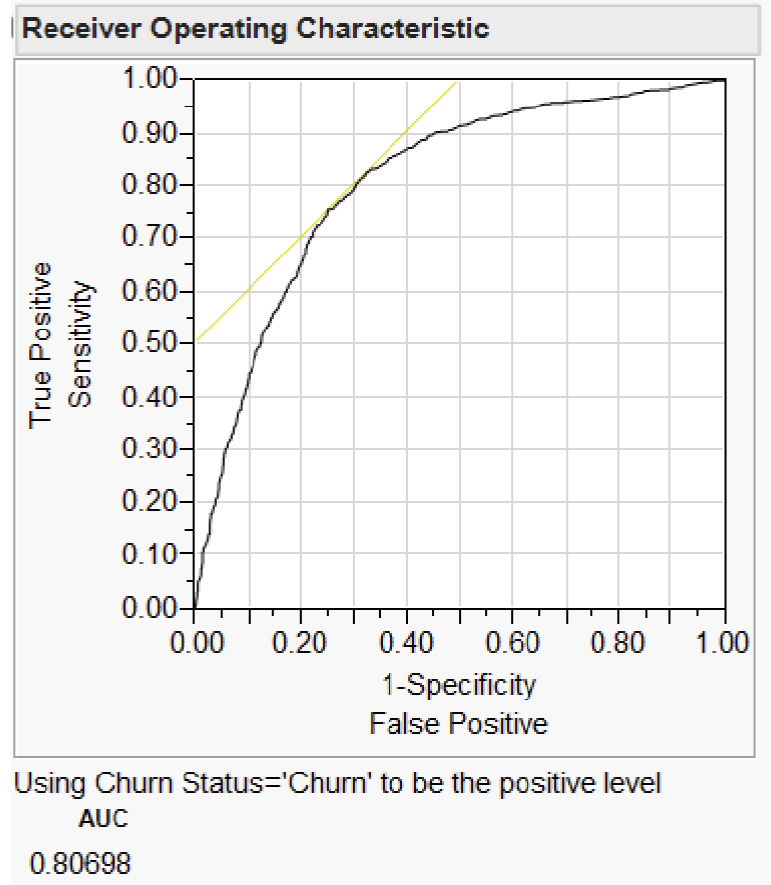
An ROC curve shows how rapidly the true positive and false negative transition happens, with the goal being to have diagnostics that maximise the area under the curve.

Two standard definitions used in predictive modelling :

• Sensitivity = the probability that a given x value (a test or measure) correctly predicts an existing condition.

• Specificity = the probability that a test correctly predicts that a condition does not exist.

A ROC curve is a plot of sensitivity by (1 – specificity) for each value of x. The area under the ROC curve is a common index used to summarize the information contained in the curve.

• In the plot, a light yellow line is drawn at a 45-degree angle tangent to the ROC Curve.

• This marks a good cutoff point under the assumption that false negatives and false positives have similar costs.

ROC values (between 0.5 and 1) provide a good indication of model performance :

• 0.5 – No distinguish ability (the model has no meaning).

• 0.51 – 0.7 – Low distinguish ability (not a very good model yet the model can be used).

• 0.71 – 0.9 – Very good distinguish ability.

• 0.91 – 1 – Excellent distinguish ability.

Warning

In some fields, logistic regression models can have an excellent distinguish ability, however this might indicate that the model is “too good to be true”.

Review the model to ensure no variables from the future or other odd parameter values.

5. GW MULTIPLE LOGISTIC REGRES MODEL

As an expansion to the standard logistic regression, Geographically Weighted Logistic Regression (GWLR) incorporates a set geographical location to the models :

logit ( p_i ) = log ( p_i / 1 - p_i ) = 𝛽₀( u_i , v_i ) + 𝛽₁( u_i , v_i )𝑥₁

where, 𝛽_0i and 𝛽_1i = local model parameters specific to location at ( u_i , v_i ) coordinate.

GWLR is the geographically weighted extension to the logistic regression model and similar to ordinary regression.

But with the help of a moving window or kernel function facility provided by geographically weighted methods, local regression models are computed at locations all over the study region.

The GWR discussed in previous lesson can be extended to GWLR with the help of a logit function as shown in the formula above.

The distance weights of GWLR are distance-based.

Two commonly used distance weights :

• fixed-distance weighted

• adaptive-distance weighted

The minimum bandwidth distance or size can be determined by :

• Akaike Information criterion (AIC)

• Cross-validation (CV)

Similar to basic gwr method, five (5) spatial kernel⁶ namely :

⁶ Exploratory Spatial Data Analysis with gwpcorMapper: an Interactive Mapping Tool for Geographically Weighted Correlation and Partial Correlation - Scientific Figure on ResearchGate. Available from: https://www.researchgate.net/figure/Kernel-functions-available-in-gwpcorMapper-a-Gaussian-b-exponential-c-box-car-d_fig2_360992908 [accessed 15 Dec, 2022]

• Gaussian,

• Exponential,

• Box-car,

• Bi-square

• Tri-cube smoothing methods

6. REFERENCES

Reading materials suggested by Prof Kam.

• Kleinbaum, D.G. and Klein, M (2010) Logistic Regression: A Self‐Learning Text (3rd Edition). Springer New York.

• Hosmer, D. W., JR. et. al (2013). Applied Logistic Regression (3rd Edition). John Wiley & Sons, Inc., Hoboken, New Jersey.

• Atkinson, P.M., German, S.E., Sear, D.Q., & Clark, M.J. (2010). Exploring the relations between riverbank erosion and geomorphological controls using geographically weighted logistic regression. Geographical Analysis, 35(1), 58 - 82. https://doi.org/10.1111/j.1538-4632.2003.tb01101.x