Geospatial Data Wrangling with R [1]

Published

November 18, 2022

Modified

March 6, 2023

1.1 OVERVIEW

Expected learning outcome

installing and loading sf and tidyverse packages into R environment,
importing geospatial data by using appropriate functions of sf package,
importing aspatial data by using appropriate function of readr package,
exploring the content of simple feature data frame by using appropriate Base R and sf functions,
assigning or transforming coordinate systems by using using appropriate sf functions,
converting an aspatial data into a sf data frame by using appropriate function of sf package,
performing geoprocessing tasks by using appropriate functions of sf package,
performing data wrangling tasks by using appropriate functions of dplyr package and
performing Exploratory Data Analysis (EDA) by using appropriate functions from ggplot2 package.

1.2 R PACKAGE REQUIRED

Following are the packages require for this exercise :

sf for importing, managing, and processing geospatial data.
tidyverse for performing data science tasks such as importing, wrangling and visualising data.
- readr for importing csv data
- readxl for importing Excel worksheet
- tidyr for manipulating data
- dplyr for transforming data
- ggplot2 for visualising data

1.2.1 Load R Packages

Usage of the code chunk below :

p_load( ) - pacman - to load packages into R environment. This function will attempt to install the package from CRAN or the pacman repository list if it is not installed.

Show the code

pacman::p_load(sf, tidyverse, readr, readxl, ggplot2, dplyr, tidyr, units)

Remarks :

sf, sp, (rgdal, rgeos both are retiring by year 2023), tidyverse, questionr, janitor, psych, ggplot2, gcookbook, tmap, ggpubr, egg, corrplot, gtsummary, regclass, caret, heatmaply, ggdendro, cluster, factoextra, spdep, ClustGeo, GGally, skimr, stringr, funModeling, knitr, caTools, viridis, rgeoda, cowplot, patchwork.

Alternate code chunk -

packages = c('tidyverse', 'sf', 'readr', 'readxl','ggplot2','dplyr','tidyr')
for(p in packages){
  if(!require(p, character.only = T)){
    install.packages(p)
  }
  library(p, character.only = T)
}

1.3 GEOSPATIAL DATA

1.3.1 Acquire Data

Data.gov.sg
- Download Master Plan 2014 Subzone Boundary (web)
- Download Pre-School Location
LTADataMall
- Download Cycling Path
Inside Airbnb
- Download the latest version of Singapore Airbnb data.

1.3.2 Import Geospatial Data

This section focus on importing dataset in shapefile format.

1.3.2.1 import Singapore boundary data

Usage of the code chunk below :

st_read( ) - sf - to read simple features for “MP14_SUBZONE_WEB_PL” and name as “mpsz”.

dsn( ) -to define the data path. DSN = data source name.
layer( ) -to provide shapefile name.

Show the code

mpsz = st_read(dsn = "data/geospatial",
               layer = "MP14_SUBZONE_WEB_PL")

Reading layer `MP14_SUBZONE_WEB_PL' from data source 
  `D:\jephOstan\ISSS624\data\geospatial' using driver `ESRI Shapefile'
Simple feature collection with 323 features and 15 fields
Geometry type: MULTIPOLYGON
Dimension:     XY
Bounding box:  xmin: 2667.538 ymin: 15748.72 xmax: 56396.44 ymax: 50256.33
Projected CRS: SVY21

Remarks :

Observations : 323 in multipolygon

CRS : Projected CRS i.e. SVY21

1.3.2.2 import polyline data for cyclingpath

Show the code

cyclingpath = st_read(dsn = "data/geospatial",                 
                      layer = "CyclingPath")

Reading layer `CyclingPath' from data source 
  `D:\jephOstan\ISSS624\data\geospatial' using driver `ESRI Shapefile'
Simple feature collection with 2248 features and 2 fields
Geometry type: MULTILINESTRING
Dimension:     XY
Bounding box:  xmin: 11854.32 ymin: 28347.98 xmax: 42626.09 ymax: 48948.15
Projected CRS: SVY21

Remarks :

Observations : 2,248 in multilinestring

CRS : Projected CRS i.e. SVY21

1.3.2.3 import GIS data in kml format for preschool

Show the code

preschool = st_read("data/geospatial/pre-schools-location-kml.kml")

Reading layer `PRESCHOOLS_LOCATION' from data source 
  `D:\jephOstan\ISSS624\data\geospatial\pre-schools-location-kml.kml' 
  using driver `KML'
Simple feature collection with 1925 features and 2 fields
Geometry type: POINT
Dimension:     XYZ
Bounding box:  xmin: 103.6824 ymin: 1.247759 xmax: 103.9897 ymax: 1.462134
z_range:       zmin: 0 zmax: 0
Geodetic CRS:  WGS 84

Remarks :

Observations : 1,925 in point

CRS : Geodetic CRS i.e. SVY21

1.3.3 Import Aspatial Data

Two (2) key functions i.e. Import and Inspect.

1.3.3.1 import aspatial data

Usage of the code chunk below :

read_csv( ) - qtl2 - to read a csv file.

Show the code

listings <- read_csv("data/aspatial/listings.csv")

Rows: 4161 Columns: 18
── Column specification ────────────────────────────────────────────────────────
Delimiter: ","
chr   (6): name, host_name, neighbourhood_group, neighbourhood, room_type, l...
dbl  (11): id, host_id, latitude, longitude, price, minimum_nights, number_o...
date  (1): last_review

ℹ Use `spec()` to retrieve the full column specification for this data.
ℹ Specify the column types or set `show_col_types = FALSE` to quiet this message.

Remarks :

Consists of 4,161 observations over 18 variables

Assume CRS as WGS84

1.3.3.2 review dataframe with list( ) function

Usage of the code chunk below :

list( ) - base - to list data.

Show the code

list(listings)

1.3.4 Create sf Data Frame

Two (2) key functions i.e. Convert and Inspect.

1.3.4.1 convert data frame

Usage of the code chunk below :

st_as_sf( ) - sf - to convert aspatial object to an sf object.

coords - provide x-coordinates first before y-coordinates.
crs - define the coordinates reference system with 4326.
%>% - to nest st_transform() to transform the newly created simple feature data frame into svy21 projected CRS.

Show the code

listings_sf <- st_as_sf(listings, 
                       coords = c("longitude", "latitude"),
                       crs = 4326) %>%
  st_transform(crs = 3414)

Remarks :

“geometry” is creaed while “longitude” and “latitude” are removed.

1.3.4.2 inspect output

Show the code

glimpse(listings_sf)

Rows: 4,161
Columns: 17
$ id                             <dbl> 50646, 71609, 71896, 71903, 275344, 289…
$ name                           <chr> "Pleasant Room along Bukit Timah", "Ens…
$ host_id                        <dbl> 227796, 367042, 367042, 367042, 1439258…
$ host_name                      <chr> "Sujatha", "Belinda", "Belinda", "Belin…
$ neighbourhood_group            <chr> "Central Region", "East Region", "East …
$ neighbourhood                  <chr> "Bukit Timah", "Tampines", "Tampines", …
$ room_type                      <chr> "Private room", "Private room", "Privat…
$ price                          <dbl> 80, 145, 85, 85, 49, 184, 79, 49, 55, 5…
$ minimum_nights                 <dbl> 92, 92, 92, 92, 60, 92, 92, 60, 60, 60,…
$ number_of_reviews              <dbl> 18, 20, 24, 47, 14, 12, 133, 17, 12, 3,…
$ last_review                    <date> 2014-12-26, 2020-01-17, 2019-10-13, 20…
$ reviews_per_month              <dbl> 0.18, 0.15, 0.18, 0.34, 0.11, 0.10, 1.0…
$ calculated_host_listings_count <dbl> 1, 6, 6, 6, 44, 6, 7, 44, 44, 44, 6, 7,…
$ availability_365               <dbl> 365, 340, 265, 365, 296, 285, 365, 181,…
$ number_of_reviews_ltm          <dbl> 0, 0, 0, 0, 1, 0, 0, 3, 2, 0, 1, 0, 0, …
$ license                        <chr> NA, NA, NA, NA, "S0399", NA, NA, "S0399…
$ geometry                       <POINT [m]> POINT (22646.02 35167.9), POINT (…

1.3.5 Retrieve Geometry List-column

There are 3 methods to do so :

mpsz$geom
mpsz[[1]]
st_geometry()

Show the code

st_geometry(mpsz)

Geometry set for 323 features 
Geometry type: MULTIPOLYGON
Dimension:     XY
Bounding box:  xmin: 2667.538 ymin: 15748.72 xmax: 56396.44 ymax: 50256.33
Projected CRS: SVY21
First 5 geometries:

MULTIPOLYGON (((31495.56 30140.01, 31980.96 296...

MULTIPOLYGON (((29092.28 30021.89, 29119.64 300...

MULTIPOLYGON (((29932.33 29879.12, 29947.32 298...

MULTIPOLYGON (((27131.28 30059.73, 27088.33 297...

MULTIPOLYGON (((26451.03 30396.46, 26440.47 303...

Show the code

mpsz$geom

Geometry set for 323 features 
Geometry type: MULTIPOLYGON
Dimension:     XY
Bounding box:  xmin: 2667.538 ymin: 15748.72 xmax: 56396.44 ymax: 50256.33
Projected CRS: SVY21
First 5 geometries:

MULTIPOLYGON (((31495.56 30140.01, 31980.96 296...

MULTIPOLYGON (((29092.28 30021.89, 29119.64 300...

MULTIPOLYGON (((29932.33 29879.12, 29947.32 298...

MULTIPOLYGON (((27131.28 30059.73, 27088.33 297...

MULTIPOLYGON (((26451.03 30396.46, 26440.47 303...

1.3.6 Reveal Variables & Data Types

Two common methods used i.e. glimpse( ) and head( ).

1.3.6.1 reveal with glimpse( ) function

Usage of the code chunk below :

glimpse( ) - dplyr - to reveals the data type of each field / variable.

Show the code

glimpse(mpsz, 60)

Rows: 323
Columns: 16
$ OBJECTID   <int> 1, 2, 3, 4, 5, 6, 7, 8, 9, 10, 11, 12, …
$ SUBZONE_NO <int> 1, 1, 3, 8, 3, 7, 9, 2, 13, 7, 12, 6, 1…
$ SUBZONE_N  <chr> "MARINA SOUTH", "PEARL'S HILL", "BOAT Q…
$ SUBZONE_C  <chr> "MSSZ01", "OTSZ01", "SRSZ03", "BMSZ08",…
$ CA_IND     <chr> "Y", "Y", "Y", "N", "N", "N", "N", "Y",…
$ PLN_AREA_N <chr> "MARINA SOUTH", "OUTRAM", "SINGAPORE RI…
$ PLN_AREA_C <chr> "MS", "OT", "SR", "BM", "BM", "BM", "BM…
$ REGION_N   <chr> "CENTRAL REGION", "CENTRAL REGION", "CE…
$ REGION_C   <chr> "CR", "CR", "CR", "CR", "CR", "CR", "CR…
$ INC_CRC    <chr> "5ED7EB253F99252E", "8C7149B9EB32EEFC",…
$ FMEL_UPD_D <date> 2014-12-05, 2014-12-05, 2014-12-05, 20…
$ X_ADDR     <dbl> 31595.84, 28679.06, 29654.96, 26782.83,…
$ Y_ADDR     <dbl> 29220.19, 29782.05, 29974.66, 29933.77,…
$ SHAPE_Leng <dbl> 5267.381, 3506.107, 1740.926, 3313.625,…
$ SHAPE_Area <dbl> 1630379.3, 559816.2, 160807.5, 595428.9…
$ geometry   <MULTIPOLYGON [m]> MULTIPOLYGON (((31495.56 3…

1.3.6.2 reveal with head( ) function

Usage of the code chunk below :

head( ) - utils - to return the first 3 rows of an object i.e. mpsz.

n = number of rows / observations to display.

Show the code

head(mpsz, n = 3)

Simple feature collection with 3 features and 15 fields
Geometry type: MULTIPOLYGON
Dimension:     XY
Bounding box:  xmin: 28160.23 ymin: 28369.47 xmax: 32362.39 ymax: 30247.18
Projected CRS: SVY21
  OBJECTID SUBZONE_NO    SUBZONE_N SUBZONE_C CA_IND      PLN_AREA_N PLN_AREA_C
1        1          1 MARINA SOUTH    MSSZ01      Y    MARINA SOUTH         MS
2        2          1 PEARL'S HILL    OTSZ01      Y          OUTRAM         OT
3        3          3    BOAT QUAY    SRSZ03      Y SINGAPORE RIVER         SR
        REGION_N REGION_C          INC_CRC FMEL_UPD_D   X_ADDR   Y_ADDR
1 CENTRAL REGION       CR 5ED7EB253F99252E 2014-12-05 31595.84 29220.19
2 CENTRAL REGION       CR 8C7149B9EB32EEFC 2014-12-05 28679.06 29782.05
3 CENTRAL REGION       CR C35FEFF02B13E0E5 2014-12-05 29654.96 29974.66
  SHAPE_Leng SHAPE_Area                       geometry
1   5267.381  1630379.3 MULTIPOLYGON (((31495.56 30...
2   3506.107   559816.2 MULTIPOLYGON (((29092.28 30...
3   1740.926   160807.5 MULTIPOLYGON (((29932.33 29...

1.4 GEODATA PROCESSING

1.4.1 Transform CRS

Ensure all dataframes are in the same projected CRS.

1.4.1.1 transform with st_set_crs( ) function

Generally, there are two main steps involved.

– retrieve CRS information

Usage of the code chunk below :

st_crs( ) - sf - to retrieve coordinate reference system for mpsz.

Show the code

st_crs(mpsz)

Coordinate Reference System:
  User input: SVY21 
  wkt:
PROJCRS["SVY21",
    BASEGEOGCRS["SVY21[WGS84]",
        DATUM["World Geodetic System 1984",
            ELLIPSOID["WGS 84",6378137,298.257223563,
                LENGTHUNIT["metre",1]],
            ID["EPSG",6326]],
        PRIMEM["Greenwich",0,
            ANGLEUNIT["Degree",0.0174532925199433]]],
    CONVERSION["unnamed",
        METHOD["Transverse Mercator",
            ID["EPSG",9807]],
        PARAMETER["Latitude of natural origin",1.36666666666667,
            ANGLEUNIT["Degree",0.0174532925199433],
            ID["EPSG",8801]],
        PARAMETER["Longitude of natural origin",103.833333333333,
            ANGLEUNIT["Degree",0.0174532925199433],
            ID["EPSG",8802]],
        PARAMETER["Scale factor at natural origin",1,
            SCALEUNIT["unity",1],
            ID["EPSG",8805]],
        PARAMETER["False easting",28001.642,
            LENGTHUNIT["metre",1],
            ID["EPSG",8806]],
        PARAMETER["False northing",38744.572,
            LENGTHUNIT["metre",1],
            ID["EPSG",8807]]],
    CS[Cartesian,2],
        AXIS["(E)",east,
            ORDER[1],
            LENGTHUNIT["metre",1,
                ID["EPSG",9001]]],
        AXIS["(N)",north,
            ORDER[2],
            LENGTHUNIT["metre",1,
                ID["EPSG",9001]]]]

– transform CRS

Usage of the code chunk below :

st_set_crs( ) - sf - to replace the coordinate reference system for mpsz.

Show the code

mpsz3414 <- st_set_crs(mpsz, 3414)

Warning: st_crs<- : replacing crs does not reproject data; use st_transform for
that

– verify CRS

Show the code

st_crs(mpsz3414)

Coordinate Reference System:
  User input: EPSG:3414 
  wkt:
PROJCRS["SVY21 / Singapore TM",
    BASEGEOGCRS["SVY21",
        DATUM["SVY21",
            ELLIPSOID["WGS 84",6378137,298.257223563,
                LENGTHUNIT["metre",1]]],
        PRIMEM["Greenwich",0,
            ANGLEUNIT["degree",0.0174532925199433]],
        ID["EPSG",4757]],
    CONVERSION["Singapore Transverse Mercator",
        METHOD["Transverse Mercator",
            ID["EPSG",9807]],
        PARAMETER["Latitude of natural origin",1.36666666666667,
            ANGLEUNIT["degree",0.0174532925199433],
            ID["EPSG",8801]],
        PARAMETER["Longitude of natural origin",103.833333333333,
            ANGLEUNIT["degree",0.0174532925199433],
            ID["EPSG",8802]],
        PARAMETER["Scale factor at natural origin",1,
            SCALEUNIT["unity",1],
            ID["EPSG",8805]],
        PARAMETER["False easting",28001.642,
            LENGTHUNIT["metre",1],
            ID["EPSG",8806]],
        PARAMETER["False northing",38744.572,
            LENGTHUNIT["metre",1],
            ID["EPSG",8807]]],
    CS[Cartesian,2],
        AXIS["northing (N)",north,
            ORDER[1],
            LENGTHUNIT["metre",1]],
        AXIS["easting (E)",east,
            ORDER[2],
            LENGTHUNIT["metre",1]],
    USAGE[
        SCOPE["Cadastre, engineering survey, topographic mapping."],
        AREA["Singapore - onshore and offshore."],
        BBOX[1.13,103.59,1.47,104.07]],
    ID["EPSG",3414]]

1.4.1.2 transform with st_transform( ) function

– transform wgs84 to svy21

Usage of the code chunk below :

st_transform( ) - sf - to reproject x from one coordinate system wgs84 to svy21 mathematically, which is not capable by st_set_crs().

Show the code

preschool3414 <- st_transform(preschool, 
                              crs = 3414)

– inspect output

Show the code

st_geometry(preschool3414)

Geometry set for 1925 features 
Geometry type: POINT
Dimension:     XYZ
Bounding box:  xmin: 11203.01 ymin: 25596.33 xmax: 45404.24 ymax: 49300.88
z_range:       zmin: 0 zmax: 0
Projected CRS: SVY21 / Singapore TM
First 5 geometries:

POINT Z (13258.34 35611.04 0)

POINT Z (35272.09 41373.42 0)

POINT Z (25050.54 46634.14 0)

POINT Z (22892.48 46127.66 0)

POINT Z (34155.79 41949.13 0)

1.4.2 Set Up Buffering

To upgrade the existing cycling path, the authority needs to acquire 5 metres of reserved land on both sides of the current cycling path.

Task : determine the extent of the land acquired and its total area.

solution :

Usage of the code chunk below :

st_buffer( ) - sf - to set geometric unary operation. - dist = to set buffer distance for cyclingpath. - nQuadSegs = to set number of segments per quadrant. !!!!! dnt understand.

Show the code

buffer_cycling <- st_buffer(cyclingpath, 
                            dist = 5, 
                            nQuadSegs = 30)

st_area( ) - sf - to compute area for buffer_cycling and assigned to new variable “area”

Show the code

buffer_cycling$area <- st_area(buffer_cycling)

sum( ) - base - to compute sum of “area” under buffer_cycling.

Show the code

sum(buffer_cycling$area)

1556978 [m^2]

1.4.3 Perform Point-in-Polygon Count

scenario : A preschool service group wants to determine the number of preschools in each Planning Subzone.

solution :

Usage of the code chunk below :

st_intersect( ) - sf - to identify pre-schools located inside each Planning Subzone.

lengths( ) - base - to calculate the number of pre-schools within each planning subzone.

Show the code

mpsz3414$preSch_count <- lengths(
  st_intersects(mpsz3414, 
                preschool3414))

summary(mpsz3414$preSch_count)

   Min. 1st Qu.  Median    Mean 3rd Qu.    Max. 
   0.00    0.00    3.00    5.96    9.00   58.00

1.4.3.1 list planning subzone with the most number of pre-school

Show the code

top_n(mpsz3414, 1, preSch_count)

Simple feature collection with 1 feature and 16 fields
Geometry type: MULTIPOLYGON
Dimension:     XY
Bounding box:  xmin: 39655.33 ymin: 35966 xmax: 42940.57 ymax: 38622.37
Projected CRS: SVY21 / Singapore TM
  OBJECTID SUBZONE_NO     SUBZONE_N SUBZONE_C CA_IND PLN_AREA_N PLN_AREA_C
1      189          2 TAMPINES EAST    TMSZ02      N   TAMPINES         TM
     REGION_N REGION_C          INC_CRC FMEL_UPD_D   X_ADDR   Y_ADDR SHAPE_Leng
1 EAST REGION       ER 21658EAAF84F4D8D 2014-12-05 41122.55 37392.39   10180.62
  SHAPE_Area                       geometry preSch_count
1    4339824 MULTIPOLYGON (((42196.76 38...           58

1.4.3.2 calculate the density of pre-school by planning subzone.

step 1 - use [st_area()] to derive the area of each planning subzone

Show the code

mpsz3414$area <- mpsz3414 %>%
  st_area()

step 2 -

Show the code

mpsz3414 <- mpsz3414 %>%
  mutate(preSch_density = preSch_count/area * 1000000)

1.5 EXPLORATORY DATA ANALYSIS (EDA)

1.5.1 Plot Histogram

1.5.1.1 plot with Graphics Function

Usage of the code chunk below :

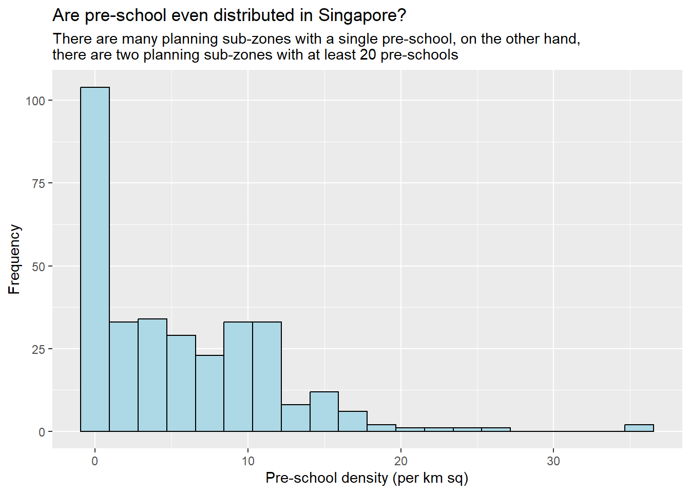
hist( ) - graphics - to reveal the distribution of “preSch_density”. Too basic for further customisation.

Show the code

hist(mpsz3414$preSch_density)

1.5.1.2 plot with ggplot2 function

Usage of the code chunk below :

geom_histogram( ) - ggplot2 - to reveal the distribution of “preSch_density”.

Show the code

ggplot(data = mpsz3414, 
       aes(x = as.numeric(preSch_density))) +
  geom_histogram(bins = 20,
                 color = "black",
                 fill = "light blue") +
  labs(title = "Are pre-school even distributed in Singapore?",
       subtitle = "There are many planning sub-zones with a single pre-school, on the other hand, \nthere are two planning sub-zones with at least 20 pre-schools",
       x = "Pre-school density (per km sq)",
       y = "Frequency")

1.5.2 Plot Scatter Plot

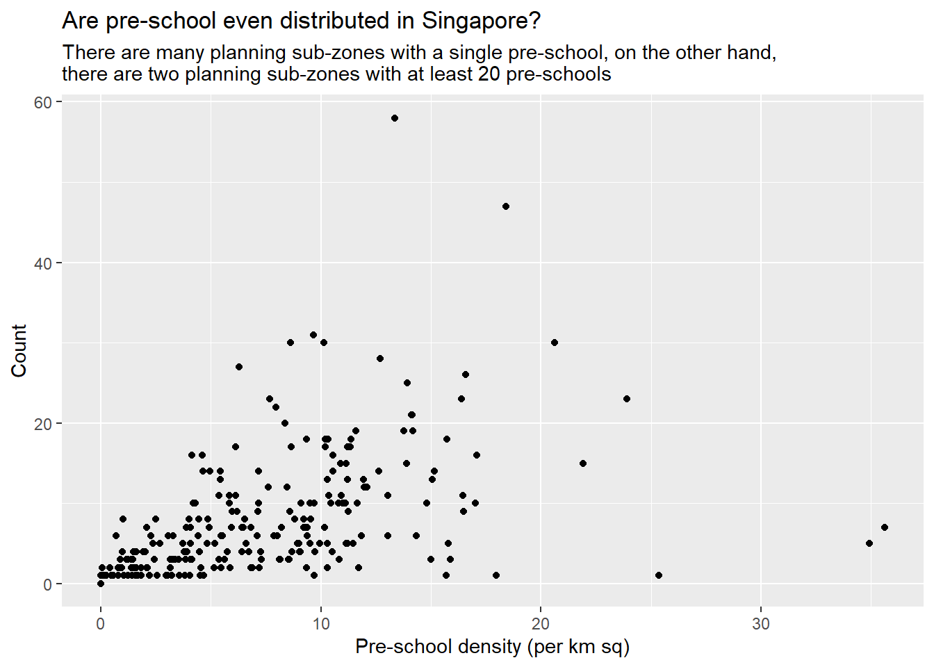
To plot a scatter plot showing the relationship between Pre-school Density and Pre-school Count.

1.5.2.1 plot with ggplot2 function

Usage of the code chunk below :

geom_point( ) - ggplot2 - to reveal the relationship between “preSch_density” and “preSch_count”.

-- display Row ID of Each Observation

Show the code

ggplot(mpsz3414, 
       aes(x = preSch_density, 
           y = preSch_count)) +
  geom_point() + 
  geom_text(label = rownames(mpsz3414))

-- change line type and colour

Show the code

ggplot(mpsz3414, 
       aes(x = preSch_density, 
           y = preSch_count)) + 
  geom_point(shape = 18, 
             color = "blue") + 
  geom_smooth(method = lm, 
              se = FALSE, 
              linetype = "dashed", 
              color = "darkred")

`geom_smooth()` using formula = 'y ~ x'

-- change colour for the Confidence Interval

Show the code

ggplot(mpsz3414,
       aes(x = preSch_density, 
           y = preSch_count)) + 
  geom_point(shape = 18, 
             color = "blue") + 
  geom_smooth(method = lm, 
              linetype = "dashed", 
              color = "darkred", 
              fill = "blue")

`geom_smooth()` using formula = 'y ~ x'

-- add title and subtitle

Show the code

ggplot(mpsz3414,
       aes(x = as.numeric(preSch_density), 
           y = (preSch_count))) + 
  geom_point() +
  labs(title = "Are pre-school even distributed in Singapore?",
       subtitle = "There are many planning sub-zones with a single pre-school, on the other hand, \nthere are two planning sub-zones with at least 20 pre-schools",
       x = "Pre-school density (per km sq)",
       y = "Count")

1.6 GEOSPATIAL VISUALISATION

Usage of the code chunk below :

plot( ) - graphics - to plot map for each field / variable in mpsz.

Show the code

plot(mpsz,
     max.plot = 15,
     asp = 1)

1.6.1 Plot Boundary

Usage of the code chunk below :

st_geometry( ) - sf - to get the map boundary for the plot( ) function.

Show the code

plot(st_geometry(mpsz))

1.6.2 Plot Specific Attribute

Show the code

plot(mpsz["PLN_AREA_N"])

1.7 References

r4gdsa.netlify.app. https://r4gdsa.netlify.app/chap02.html#data-preparation
STHDA (Statistical tools for high-throughput data analysis), (N.A.), ggplot2 scatter plots : Quick start guide - R software and data visualization. http://www.sthda.com/english/wiki/ggplot2-scatter-plots-quick-start-guide-r-software-and-data-visualization