Explore2 : Thematic Mapping

Published

January 16, 2023

Modified

March 6, 2023

1 OVERVIEW

Expected learning outcome

installing and loading sf and tidyverse packages into R environment,
importing geospatial data by using appropriate functions of sf package,
importing aspatial data by using appropriate function of readr package,
exploring the content of simple feature data frame by using appropriate Base R and sf functions,
assigning or transforming coordinate systems by using using appropriate sf functions,
converting an aspatial data into a sf data frame by using appropriate function of sf package,
performing geoprocessing tasks by using appropriate functions of sf package,
performing data wrangling tasks by using appropriate functions of dplyr package and
performing Exploratory Data Analysis (EDA) by using appropriate functions from ggplot2 package.

2. R PACKAGE REQUIRED

Following are the packages require for this exercise :

sf for importing, managing, and processing geospatial data.
tidyverse for performing data science tasks such as importing, wrangling and visualising data.
- readr for importing csv data
- readxl for importing Excel worksheet
- tidyr for manipulating data
- dplyr for transforming data
- ggplot2 for visualising data

2.1 Load R Packages

Usage of the code chunk below :

p_load( ) - pacman - to load packages into R environment. This function will attempt to install the package from CRAN or the pacman repository list if it is not installed.

Show the code

pacman::p_load(sf, tidyverse, readr, readxl, ggplot2, dplyr, tidyr, units)

Remarks :

sf, sp, (rgdal, rgeos both are retiring by year 2023), tidyverse, questionr, janitor, psych, ggplot2, gcookbook, tmap, ggpubr, egg, corrplot, gtsummary, regclass, caret, heatmaply, ggdendro, cluster, factoextra, spdep, ClustGeo, GGally, skimr, stringr, funModeling, knitr, caTools, viridis, rgeoda, cowplot, patchwork.

Alternate code chunk -

packages = c('tidyverse', 'sf', 'readr', 'readxl','ggplot2','dplyr','tidyr')
for(p in packages){
  if(!require(p, character.only = T)){
    install.packages(p)
  }
  library(p, character.only = T)
}

3. GEOSPATIAL DATA

3.1 Acquire Data

Aspatial Data
1. Download the Nigeria data set in shapefile format via Access WPdx+ Global Data Repository from WPdx Global Data Repositories.
2. Rename the title of the data set to “geo_export”.

Note

The file size of the downloaded data is about 422 MB due to water points data from multiple countries.

-   [Such file size may require extra effort and time to manage the code chunks and files in the R environment before pushing them to GitHub.]{style="color:#d69c3c"}

[Hence, to avoid any error in pushing files larger than 100 MB to Git, filtered Nigeria water points and removed unnecessary variables before uploading into the R environment.]{style="color:#d69c3c"}

[Therewith, the CSV file size should be lesser than 100 MB.]{style="color:#d69c3c"}

Geospatial Data
1. Download the Nigeria geoBoundaries data set at ADM2 level¹ from geoBoundaries.org or the Humanitarian Data Exchange portal.
2. Rename the title of the data set to “nga_admbnda_adm2_osgof_20190417”

3.2 Import Data

3.2.1 Import Boundary Data

Included two extra functions when importing the data :

transform the boundary data to “26392”
check parsing error.

3.2.1.1 import data

bdy_nga.sf <- st_read(dsn = "data/geospatial",
               layer = "geoBoundaries-NGA-ADM2") %>%
  select(shapeName) %>%
  st_transform(crs = 26392)

Reading layer `geoBoundaries-NGA-ADM2' from data source 
  `D:\jephOstan\ISSS624\exploration\exploration_2\data\geospatial' 
  using driver `ESRI Shapefile'
Simple feature collection with 774 features and 5 fields
Geometry type: MULTIPOLYGON
Dimension:     XY
Bounding box:  xmin: 2.668534 ymin: 4.273007 xmax: 14.67882 ymax: 13.89442
Geodetic CRS:  WGS 84

problems(bdy_nga.sf)

Remarks :

Observations : 774 in multipolygon

CRS : Projected CRS i.e. WGS 84

3.2.1.2 save sf data frame into RDS format

Show the code

write_rds(bdy_nga.sf,
          "data/geodata/bdy_nga.sf.rds")

3.2.1.3 read RDS file

bdy_nga.sf <- read_rds("data/geodata/bdy_nga.sf.rds")

3.2.2 Import Attribute Data

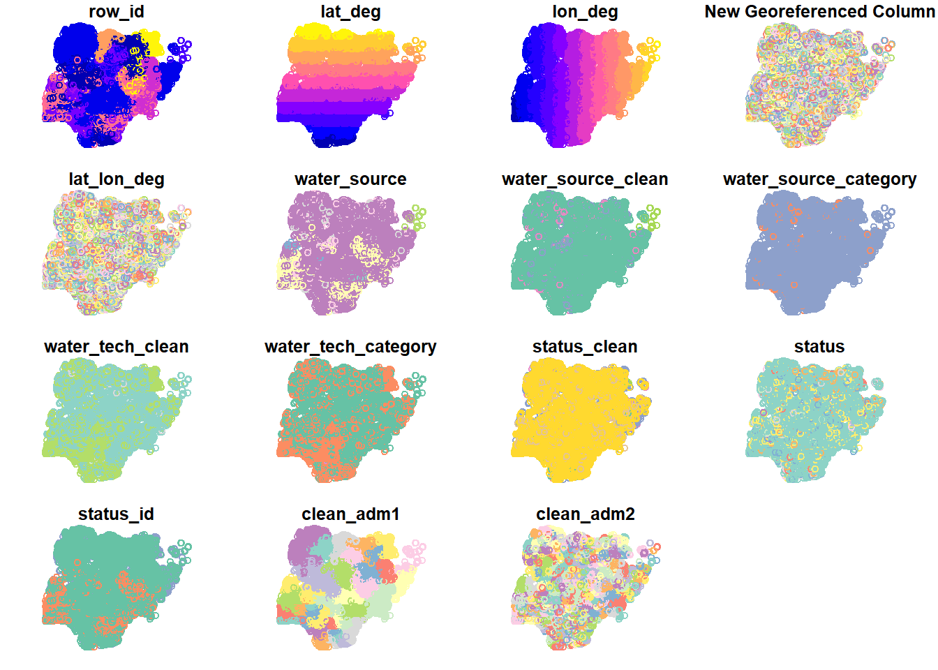
wp_attribute <- read_csv("data/aspatial/WPdx_NGAv1.2.1.csv",
                       col_select = c(`row_id`,
                                      `#lat_deg`,
                                      `#lon_deg`,
                                      `New Georeferenced Column`,
                                      `lat_lon_deg`,
                                      `#water_source`,
                                      `#water_source_clean`,
                                      `#water_source_category`,
                                      `#water_tech_clean`,
                                      `#water_tech_category`,
                                      `#status_clean`,
                                      `#status`,
                                      `#status_id`,
                                      `#clean_adm1`,
                                      `#clean_adm2`,
                                      `water_point_population`,
                                      `local_population_1km`,
                                      `crucialness_score`,
                                      `pressure_score`,
                                      `usage_capacity`,
                                      `staleness_score`,
                                      `rehab_priority`,
                                      `is_urban`)) %>%
  rename(lat_deg = `#lat_deg`, 
         lon_deg = `#lon_deg`,
         water_source = `#water_source`,
         water_source_clean = `#water_source_clean`, 
         water_source_category = `#water_source_category`, 
         water_tech_clean = `#water_tech_clean`, 
         water_tech_category = `#water_tech_category`,
         status_clean = `#status_clean`,
         status = `#status`,
         status_id = `#status_id`,
         clean_adm1 = `#clean_adm1`,
         clean_adm2 = `#clean_adm2`)

Rows: 95008 Columns: 23
── Column specification ────────────────────────────────────────────────────────
Delimiter: ","
chr (12): #status_id, #water_source_clean, #water_source_category, #water_te...
dbl (10): row_id, #lat_deg, #lon_deg, rehab_priority, water_point_population...
lgl  (1): is_urban

ℹ Use `spec()` to retrieve the full column specification for this data.
ℹ Specify the column types or set `show_col_types = FALSE` to quiet this message.

problems(wp_attribute)

3.2.2.1 inspect for missing value

Show the code

skimr::skim(wp_attribute)

Data summary
Name	wp_attribute
Number of rows	95008
Number of columns	23
_______________________
Column type frequency:
character	12
logical	1
numeric	10
________________________
Group variables	None

Variable type: character

skim_variable	n_missing	complete_rate	min	max	n_unique
New Georeferenced Column	0	1.00	11	45	95008
lat_lon_deg	0	1.00	8	42	95008
water_source	0	1.00	3	32	16
water_source_clean	302	1.00	8	22	5
water_source_category	302	1.00	4	11	3
water_tech_clean	10055	0.89	8	26	11
water_tech_category	10055	0.89	8	15	4
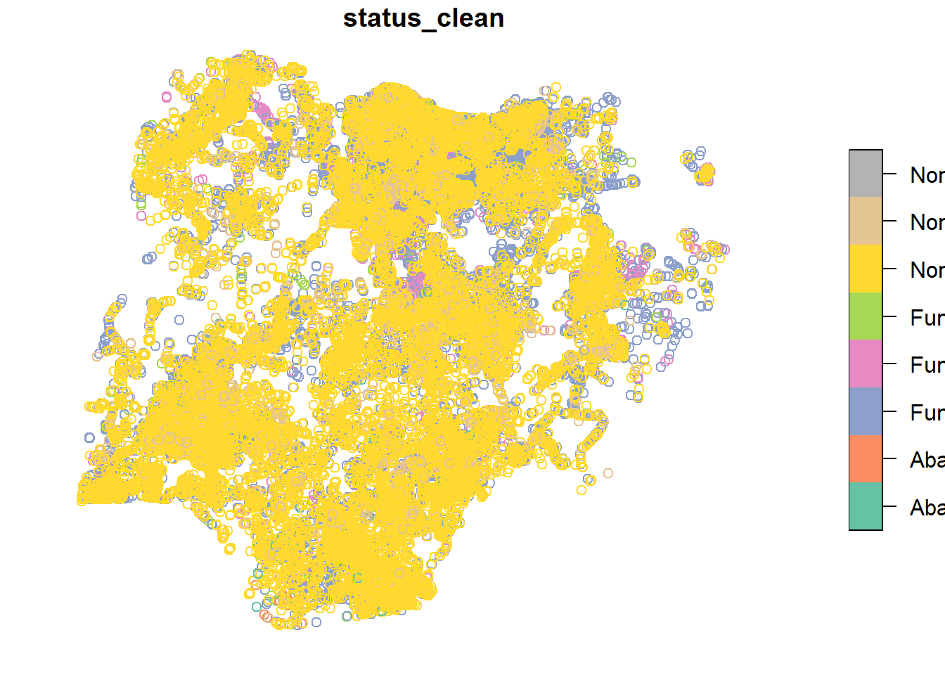
status_clean	10656	0.89	9	32	8
status	10656	0.89	14	156	834
status_id	0	1.00	2	7	3
clean_adm1	0	1.00	3	25	37
clean_adm2	0	1.00	3	19	753

Variable type: logical

skim_variable	n_missing	complete_rate	mean	count
is_urban	0	1	0.21	FAL: 75444, TRU: 19564

Variable type: numeric

skim_variable	n_missing	complete_rate	mean	sd	p0	p25	p50	p75	p100	hist
row_id	0	1.00	199975.48	189726.13	10732.00	52632.75	86952.50	323671.50	681838.00	▇▃▂▂▁
lat_deg	0	1.00	9.33	2.48	4.30	7.36	9.09	11.83	13.87	▃▇▅▅▆
lon_deg	0	1.00	7.50	2.25	2.71	5.52	7.89	9.08	14.22	▃▃▇▃▁
water_point_population	539	0.99	1246.32	4027.41	0.00	117.00	413.00	1169.00	384595.00	▇▁▁▁▁
local_population_1km	539	0.99	3723.15	7417.59	0.00	597.00	1756.00	4393.00	384595.00	▇▁▁▁▁
crucialness_score	6879	0.93	0.41	0.34	0.00	0.13	0.30	0.63	1.00	▇▅▃▁▅
pressure_score	6879	0.93	3.21	9.04	0.00	0.40	1.18	3.10	776.97	▇▁▁▁▁
usage_capacity	0	1.00	488.63	310.95	50.00	300.00	300.00	1000.00	1000.00	▁▇▁▁▃
staleness_score	0	1.00	44.94	6.29	23.13	41.49	42.87	44.34	99.00	▁▇▁▁▁
rehab_priority	53109	0.44	1545.45	5243.53	0.00	136.50	522.00	1527.00	384595.00	▇▁▁▁▁

Remarks :

Observation : 95,008 water points

Variable : Out of 23 variables, there are 7 variables with missing value n percent.

3.2.2.2 derive “geometry” variable

Show the code

wp_attribute$geometry = st_as_sfc(wp_attribute$`New Georeferenced Column`)

Remarks :

Need to have “geometry” variable, else will encounter the following error -

” Error in st_sf(wp_attribute, crs = 26392) : no simple features geometry column present ”

3.2.2.3 convert to sf data frame

Show the code

wp.sf<- st_sf(wp_attribute, 
              crs = 26392)
st_crs(wp.sf)

Coordinate Reference System:
  User input: EPSG:26392 
  wkt:
PROJCRS["Minna / Nigeria Mid Belt",
    BASEGEOGCRS["Minna",
        DATUM["Minna",
            ELLIPSOID["Clarke 1880 (RGS)",6378249.145,293.465,
                LENGTHUNIT["metre",1]]],
        PRIMEM["Greenwich",0,
            ANGLEUNIT["degree",0.0174532925199433]],
        ID["EPSG",4263]],
    CONVERSION["Nigeria Mid Belt",
        METHOD["Transverse Mercator",
            ID["EPSG",9807]],
        PARAMETER["Latitude of natural origin",4,
            ANGLEUNIT["degree",0.0174532925199433],
            ID["EPSG",8801]],
        PARAMETER["Longitude of natural origin",8.5,
            ANGLEUNIT["degree",0.0174532925199433],
            ID["EPSG",8802]],
        PARAMETER["Scale factor at natural origin",0.99975,
            SCALEUNIT["unity",1],
            ID["EPSG",8805]],
        PARAMETER["False easting",670553.98,
            LENGTHUNIT["metre",1],
            ID["EPSG",8806]],
        PARAMETER["False northing",0,
            LENGTHUNIT["metre",1],
            ID["EPSG",8807]]],
    CS[Cartesian,2],
        AXIS["(E)",east,
            ORDER[1],
            LENGTHUNIT["metre",1]],
        AXIS["(N)",north,
            ORDER[2],
            LENGTHUNIT["metre",1]],
    USAGE[
        SCOPE["Engineering survey, topographic mapping."],
        AREA["Nigeria between 6°30'E and 10°30'E, onshore and offshore shelf."],
        BBOX[3.57,6.5,13.53,10.51]],
    ID["EPSG",26392]]

3.2.2.4 write sf data frame into RDS format

write_rds(wp.sf,
          "data/geodata/wp.sf.rds",
          compress = "xz")

3.2.2.5 read RDS file

wp.sf <- read_rds("data/geodata/wp.sf.rds")

3.3 Data Wrangling

3.3.1 Ensure Unique References

In order to use “shapeName” as the unique reference id, the duplicated shapeName will be append with state name respectively to become unique value.

3.3.1.1 update “shapeName” with list of row id

Show the code

bdy_nga.sf$shapeName[c(94,95,304,305,355,356,519,520,546,547,693,694)] <- 
  c("Bassa Kogi",
    "Bassa Plateau",
    "Ifelodun Kwara",
    "Ifelodun Osun",
    "Irepodun Kwara",
    "Irepodun Osun",
    "Nasarawa Kano",
    "Nasarawa Nasarawa",
    "Obi Nasarawa",
    "Obi Benue",
    "Surulere Lagos",
    "Surulere Oyo")

bdy_nga.sf$shapeName[c(94,95,304,305,355,356,519,520,546,547,693,694)]

 [1] "Bassa Kogi"        "Bassa Plateau"     "Ifelodun Kwara"   
 [4] "Ifelodun Osun"     "Irepodun Kwara"    "Irepodun Osun"    
 [7] "Nasarawa Kano"     "Nasarawa Nasarawa" "Obi Nasarawa"     
[10] "Obi Benue"         "Surulere Lagos"    "Surulere Oyo"

3.3.1.2 varify output

Usage of the code chunk below : The codechunk below is to verify the output from previous step.

Show the code

dupl_shapeName_val.sf <- bdy_nga.sf %>%
  add_count(bdy_nga.sf$shapeName) %>%
  filter(n != 1) %>%
  select(-n)

dupl_shapeName_val.sf

Simple feature collection with 0 features and 2 fields
Bounding box:  xmin: NA ymin: NA xmax: NA ymax: NA
Projected CRS: Minna / Nigeria Mid Belt
[1] shapeName            bdy_nga.sf$shapeName geometry            
<0 rows> (or 0-length row.names)

3.3.2 Perform Point-in-Polygon Overlay

Compare different approaches in combining the attribute and boundary of the water points into a simple feature object :

x	y	left
wp.sf	bdy_nga.sf	TRUE
wp.sf	bdy_nga.sf	NULL
bdy_nga.sf	wp.sf	NULL

3.3.2.1 join objects :: wp.sf, bdy_nga.sf

Show the code

wp_point.left <- st_join(x = wp.sf,
                     y = bdy_nga.sf,
                     join = st_intersects,
                     left = TRUE)

st_geometry(wp_point.left)

Geometry set for 95008 features 
Geometry type: POINT
Dimension:     XY
Bounding box:  xmin: 2.707441 ymin: 4.301812 xmax: 14.21828 ymax: 13.86568
Projected CRS: Minna / Nigeria Mid Belt
First 5 geometries:

POINT (10.47318 10.60104)

POINT (6.95009 6.78599)

POINT (7.615451 6.799595)

POINT (7.30539 6.30817)

POINT (10.44625 10.50681)

Show the code

wp_point <- st_join(x = wp.sf,
                     y = bdy_nga.sf,
                     join = st_intersects)

st_geometry(wp_point)

Geometry set for 95008 features 
Geometry type: POINT
Dimension:     XY
Bounding box:  xmin: 2.707441 ymin: 4.301812 xmax: 14.21828 ymax: 13.86568
Projected CRS: Minna / Nigeria Mid Belt
First 5 geometries:

POINT (10.47318 10.60104)

POINT (6.95009 6.78599)

POINT (7.615451 6.799595)

POINT (7.30539 6.30817)

POINT (10.44625 10.50681)

Show the code

wp_mpolygon <- st_join(x = bdy_nga.sf,
                     y = wp.sf,
                     join = st_intersects,
                     left = TRUE)

st_geometry(wp_mpolygon)

Geometry set for 774 features 
Geometry type: MULTIPOLYGON
Dimension:     XY
Bounding box:  xmin: 26662.71 ymin: 30523.38 xmax: 1344157 ymax: 1096029
Projected CRS: Minna / Nigeria Mid Belt
First 5 geometries:

MULTIPOLYGON (((548795.5 119641, 548687.4 11968...

MULTIPOLYGON (((541412.3 122192.3, 541544.6 122...

MULTIPOLYGON (((1248985 1048169, 1247285 104795...

MULTIPOLYGON (((510864.9 578541.6, 508736.2 577...

MULTIPOLYGON (((594269 120968.5, 594389.6 12087...

https://cengel.github.io/R-spatial/spatialops.html

3.3.2.2 save and read RDS Files

Show the code

write_rds(wp_point,
          "data/geodata/wp_point.rds")

Show the code

wp_point <- read_rds("data/geodata/wp_point.rds")

4. GEOSPATIAL VISUALISATION

4.1 Plot with graphics package

Usage of the code chunk below :

plot( ) - graphics - to plot map for each field / variable in mpsz.

Show the code

plot(wp_point,
     max.plot = 15,
     asp = 1)

4.2 Plot with sf package

4.2.1 Plot Boundary

Usage of the code chunk below :

st_geometry( ) - sf - to get the map boundary for the plot( ) function.

Show the code

plot(st_geometry(wp_point))

4.2.2 Plot Specific Attribute

Show the code

plot(wp_point["status_clean"])

5. REFERENCES

r4gdsa.netlify.app. https://r4gdsa.netlify.app/chap02.html#data-preparation
STHDA (Statistical tools for high-throughput data analysis), (N.A.), ggplot2 scatter plots : Quick start guide - R software and data visualization. http://www.sthda.com/english/wiki/ggplot2-scatter-plots-quick-start-guide-r-software-and-data-visualization

Footnotes

Runfola, D. et al. (2020) geoBoundaries: A global database of political administrative boundaries. PLoS ONE 15(4): e0231866. https://doi.org/10.1371/journal.pone.0231866↩︎